pacman::p_load(maptools, sf, raster, spatstat, tmap)Hands-On Exercise 04B
Importing spatial data
childcare_sf <- st_read("data/child-care-services-geojson.geojson") %>%
st_transform(crs = 3414)Reading layer `child-care-services-geojson' from data source
`C:\xinyeehow\IS415-GAA\Hands-On_Ex\Hands-On_Ex04\data\child-care-services-geojson.geojson'
using driver `GeoJSON'
Simple feature collection with 1545 features and 2 fields
Geometry type: POINT
Dimension: XYZ
Bounding box: xmin: 103.6824 ymin: 1.248403 xmax: 103.9897 ymax: 1.462134
z_range: zmin: 0 zmax: 0
Geodetic CRS: WGS 84sg_sf <- st_read(dsn = "data", layer="CostalOutline") %>%
st_transform(crs = 3414)Reading layer `CostalOutline' from data source
`C:\xinyeehow\IS415-GAA\Hands-On_Ex\Hands-On_Ex04\data' using driver `ESRI Shapefile'
Simple feature collection with 60 features and 4 fields
Geometry type: POLYGON
Dimension: XY
Bounding box: xmin: 2663.926 ymin: 16357.98 xmax: 56047.79 ymax: 50244.03
Projected CRS: SVY21st_crs(sg_sf)Coordinate Reference System:
User input: EPSG:3414
wkt:
PROJCRS["SVY21 / Singapore TM",
BASEGEOGCRS["SVY21",
DATUM["SVY21",
ELLIPSOID["WGS 84",6378137,298.257223563,
LENGTHUNIT["metre",1]]],
PRIMEM["Greenwich",0,
ANGLEUNIT["degree",0.0174532925199433]],
ID["EPSG",4757]],
CONVERSION["Singapore Transverse Mercator",
METHOD["Transverse Mercator",
ID["EPSG",9807]],
PARAMETER["Latitude of natural origin",1.36666666666667,
ANGLEUNIT["degree",0.0174532925199433],
ID["EPSG",8801]],
PARAMETER["Longitude of natural origin",103.833333333333,
ANGLEUNIT["degree",0.0174532925199433],
ID["EPSG",8802]],
PARAMETER["Scale factor at natural origin",1,
SCALEUNIT["unity",1],
ID["EPSG",8805]],
PARAMETER["False easting",28001.642,
LENGTHUNIT["metre",1],
ID["EPSG",8806]],
PARAMETER["False northing",38744.572,
LENGTHUNIT["metre",1],
ID["EPSG",8807]]],
CS[Cartesian,2],
AXIS["northing (N)",north,
ORDER[1],
LENGTHUNIT["metre",1]],
AXIS["easting (E)",east,
ORDER[2],
LENGTHUNIT["metre",1]],
USAGE[
SCOPE["Cadastre, engineering survey, topographic mapping."],
AREA["Singapore - onshore and offshore."],
BBOX[1.13,103.59,1.47,104.07]],
ID["EPSG",3414]]mpsz_sf <- st_read(dsn = "data",
layer = "MP14_SUBZONE_WEB_PL") %>%
st_transform(crs = 3414)Reading layer `MP14_SUBZONE_WEB_PL' from data source
`C:\xinyeehow\IS415-GAA\Hands-On_Ex\Hands-On_Ex04\data' using driver `ESRI Shapefile'
Simple feature collection with 323 features and 15 fields
Geometry type: MULTIPOLYGON
Dimension: XY
Bounding box: xmin: 2667.538 ymin: 15748.72 xmax: 56396.44 ymax: 50256.33
Projected CRS: SVY21tmap_mode('view')tm_shape(childcare_sf)+
tm_dots()tmap_mode('plot')Converting sf data frames to sp’s Spatial* class
childcare <- as_Spatial(childcare_sf)
mpsz <- as_Spatial(mpsz_sf)
sg <- as_Spatial(sg_sf)Converting the Spatial* class into generic sp format
childcare_sp <- as(childcare, "SpatialPoints")
sg_sp <- as(sg, "SpatialPolygons")childcare_spclass : SpatialPoints
features : 1545
extent : 11203.01, 45404.24, 25667.6, 49300.88 (xmin, xmax, ymin, ymax)
crs : +proj=tmerc +lat_0=1.36666666666667 +lon_0=103.833333333333 +k=1 +x_0=28001.642 +y_0=38744.572 +ellps=WGS84 +towgs84=0,0,0,0,0,0,0 +units=m +no_defs sg_spclass : SpatialPolygons
features : 60
extent : 2663.926, 56047.79, 16357.98, 50244.03 (xmin, xmax, ymin, ymax)
crs : +proj=tmerc +lat_0=1.36666666666667 +lon_0=103.833333333333 +k=1 +x_0=28001.642 +y_0=38744.572 +ellps=WGS84 +towgs84=0,0,0,0,0,0,0 +units=m +no_defs Converting the generic sp format into spatstat’s ppp format
childcare_ppp <- as(childcare_sp, "ppp")
childcare_pppPlanar point pattern: 1545 points
window: rectangle = [11203.01, 45404.24] x [25667.6, 49300.88] unitsplot(childcare_ppp)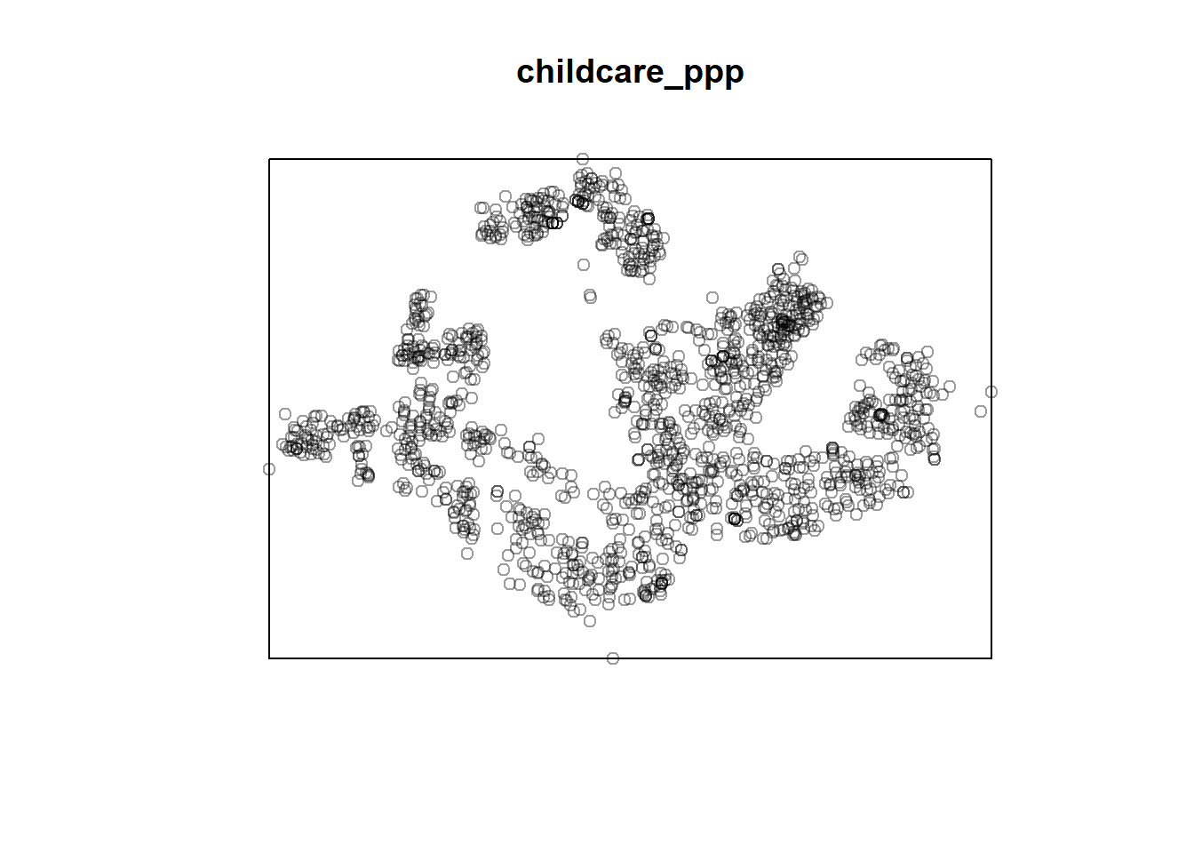
summary(childcare_ppp)Planar point pattern: 1545 points
Average intensity 1.91145e-06 points per square unit
*Pattern contains duplicated points*
Coordinates are given to 3 decimal places
i.e. rounded to the nearest multiple of 0.001 units
Window: rectangle = [11203.01, 45404.24] x [25667.6, 49300.88] units
(34200 x 23630 units)
Window area = 808287000 square unitsHandling Duplicates
any(duplicated(childcare_ppp))[1] TRUEsum(multiplicity(childcare_ppp) > 1)[1] 128tmap_mode('view')tm_shape(childcare) +
tm_dots(alpha=0.4,
size=0.05)tmap_mode('plot')childcare_ppp_jit <- rjitter(childcare_ppp,
retry=TRUE,
nsim=1,
drop=TRUE)any(duplicated(childcare_ppp_jit))[1] FALSECreating owin object
sg_owin <- as(sg_sp, "owin")plot(sg_owin)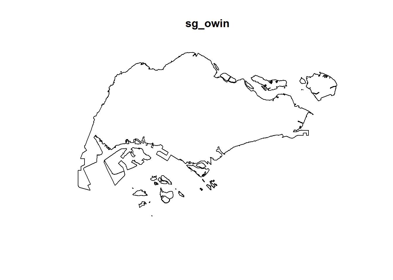
summary(sg_owin)Window: polygonal boundary
60 separate polygons (no holes)
vertices area relative.area
polygon 1 38 1.56140e+04 2.09e-05
polygon 2 735 4.69093e+06 6.27e-03
polygon 3 49 1.66986e+04 2.23e-05
polygon 4 76 3.12332e+05 4.17e-04
polygon 5 5141 6.36179e+08 8.50e-01
polygon 6 42 5.58317e+04 7.46e-05
polygon 7 67 1.31354e+06 1.75e-03
polygon 8 15 4.46420e+03 5.96e-06
polygon 9 14 5.46674e+03 7.30e-06
polygon 10 37 5.26194e+03 7.03e-06
polygon 11 53 3.44003e+04 4.59e-05
polygon 12 74 5.82234e+04 7.78e-05
polygon 13 69 5.63134e+04 7.52e-05
polygon 14 143 1.45139e+05 1.94e-04
polygon 15 165 3.38736e+05 4.52e-04
polygon 16 130 9.40465e+04 1.26e-04
polygon 17 19 1.80977e+03 2.42e-06
polygon 18 16 2.01046e+03 2.69e-06
polygon 19 93 4.30642e+05 5.75e-04
polygon 20 90 4.15092e+05 5.54e-04
polygon 21 721 1.92795e+06 2.57e-03
polygon 22 330 1.11896e+06 1.49e-03
polygon 23 115 9.28394e+05 1.24e-03
polygon 24 37 1.01705e+04 1.36e-05
polygon 25 25 1.66227e+04 2.22e-05
polygon 26 10 2.14507e+03 2.86e-06
polygon 27 190 2.02489e+05 2.70e-04
polygon 28 175 9.25904e+05 1.24e-03
polygon 29 1993 9.99217e+06 1.33e-02
polygon 30 38 2.42492e+04 3.24e-05
polygon 31 24 6.35239e+03 8.48e-06
polygon 32 53 6.35791e+05 8.49e-04
polygon 33 41 1.60161e+04 2.14e-05
polygon 34 22 2.54368e+03 3.40e-06
polygon 35 30 1.08382e+04 1.45e-05
polygon 36 327 2.16921e+06 2.90e-03
polygon 37 111 6.62927e+05 8.85e-04
polygon 38 90 1.15991e+05 1.55e-04
polygon 39 98 6.26829e+04 8.37e-05
polygon 40 415 3.25384e+06 4.35e-03
polygon 41 222 1.51142e+06 2.02e-03
polygon 42 107 6.33039e+05 8.45e-04
polygon 43 7 2.48299e+03 3.32e-06
polygon 44 17 3.28303e+04 4.38e-05
polygon 45 26 8.34758e+03 1.11e-05
polygon 46 177 4.67446e+05 6.24e-04
polygon 47 16 3.19460e+03 4.27e-06
polygon 48 15 4.87296e+03 6.51e-06
polygon 49 66 1.61841e+04 2.16e-05
polygon 50 149 5.63430e+06 7.53e-03
polygon 51 609 2.62570e+07 3.51e-02
polygon 52 8 7.82256e+03 1.04e-05
polygon 53 976 2.33447e+07 3.12e-02
polygon 54 55 8.25379e+04 1.10e-04
polygon 55 976 2.33447e+07 3.12e-02
polygon 56 61 3.33449e+05 4.45e-04
polygon 57 6 1.68410e+04 2.25e-05
polygon 58 4 9.45963e+03 1.26e-05
polygon 59 46 6.99702e+05 9.35e-04
polygon 60 13 7.00873e+04 9.36e-05
enclosing rectangle: [2663.93, 56047.79] x [16357.98, 50244.03] units
(53380 x 33890 units)
Window area = 748741000 square units
Fraction of frame area: 0.414Combining point events object and owin object
childcareSG_ppp = childcare_ppp[sg_owin]summary(childcareSG_ppp)Planar point pattern: 1545 points
Average intensity 2.063463e-06 points per square unit
*Pattern contains duplicated points*
Coordinates are given to 3 decimal places
i.e. rounded to the nearest multiple of 0.001 units
Window: polygonal boundary
60 separate polygons (no holes)
vertices area relative.area
polygon 1 38 1.56140e+04 2.09e-05
polygon 2 735 4.69093e+06 6.27e-03
polygon 3 49 1.66986e+04 2.23e-05
polygon 4 76 3.12332e+05 4.17e-04
polygon 5 5141 6.36179e+08 8.50e-01
polygon 6 42 5.58317e+04 7.46e-05
polygon 7 67 1.31354e+06 1.75e-03
polygon 8 15 4.46420e+03 5.96e-06
polygon 9 14 5.46674e+03 7.30e-06
polygon 10 37 5.26194e+03 7.03e-06
polygon 11 53 3.44003e+04 4.59e-05
polygon 12 74 5.82234e+04 7.78e-05
polygon 13 69 5.63134e+04 7.52e-05
polygon 14 143 1.45139e+05 1.94e-04
polygon 15 165 3.38736e+05 4.52e-04
polygon 16 130 9.40465e+04 1.26e-04
polygon 17 19 1.80977e+03 2.42e-06
polygon 18 16 2.01046e+03 2.69e-06
polygon 19 93 4.30642e+05 5.75e-04
polygon 20 90 4.15092e+05 5.54e-04
polygon 21 721 1.92795e+06 2.57e-03
polygon 22 330 1.11896e+06 1.49e-03
polygon 23 115 9.28394e+05 1.24e-03
polygon 24 37 1.01705e+04 1.36e-05
polygon 25 25 1.66227e+04 2.22e-05
polygon 26 10 2.14507e+03 2.86e-06
polygon 27 190 2.02489e+05 2.70e-04
polygon 28 175 9.25904e+05 1.24e-03
polygon 29 1993 9.99217e+06 1.33e-02
polygon 30 38 2.42492e+04 3.24e-05
polygon 31 24 6.35239e+03 8.48e-06
polygon 32 53 6.35791e+05 8.49e-04
polygon 33 41 1.60161e+04 2.14e-05
polygon 34 22 2.54368e+03 3.40e-06
polygon 35 30 1.08382e+04 1.45e-05
polygon 36 327 2.16921e+06 2.90e-03
polygon 37 111 6.62927e+05 8.85e-04
polygon 38 90 1.15991e+05 1.55e-04
polygon 39 98 6.26829e+04 8.37e-05
polygon 40 415 3.25384e+06 4.35e-03
polygon 41 222 1.51142e+06 2.02e-03
polygon 42 107 6.33039e+05 8.45e-04
polygon 43 7 2.48299e+03 3.32e-06
polygon 44 17 3.28303e+04 4.38e-05
polygon 45 26 8.34758e+03 1.11e-05
polygon 46 177 4.67446e+05 6.24e-04
polygon 47 16 3.19460e+03 4.27e-06
polygon 48 15 4.87296e+03 6.51e-06
polygon 49 66 1.61841e+04 2.16e-05
polygon 50 149 5.63430e+06 7.53e-03
polygon 51 609 2.62570e+07 3.51e-02
polygon 52 8 7.82256e+03 1.04e-05
polygon 53 976 2.33447e+07 3.12e-02
polygon 54 55 8.25379e+04 1.10e-04
polygon 55 976 2.33447e+07 3.12e-02
polygon 56 61 3.33449e+05 4.45e-04
polygon 57 6 1.68410e+04 2.25e-05
polygon 58 4 9.45963e+03 1.26e-05
polygon 59 46 6.99702e+05 9.35e-04
polygon 60 13 7.00873e+04 9.36e-05
enclosing rectangle: [2663.93, 56047.79] x [16357.98, 50244.03] units
(53380 x 33890 units)
Window area = 748741000 square units
Fraction of frame area: 0.414plot(sg_owin, col='light blue')
points(childcareSG_ppp, col='black', cex=.5)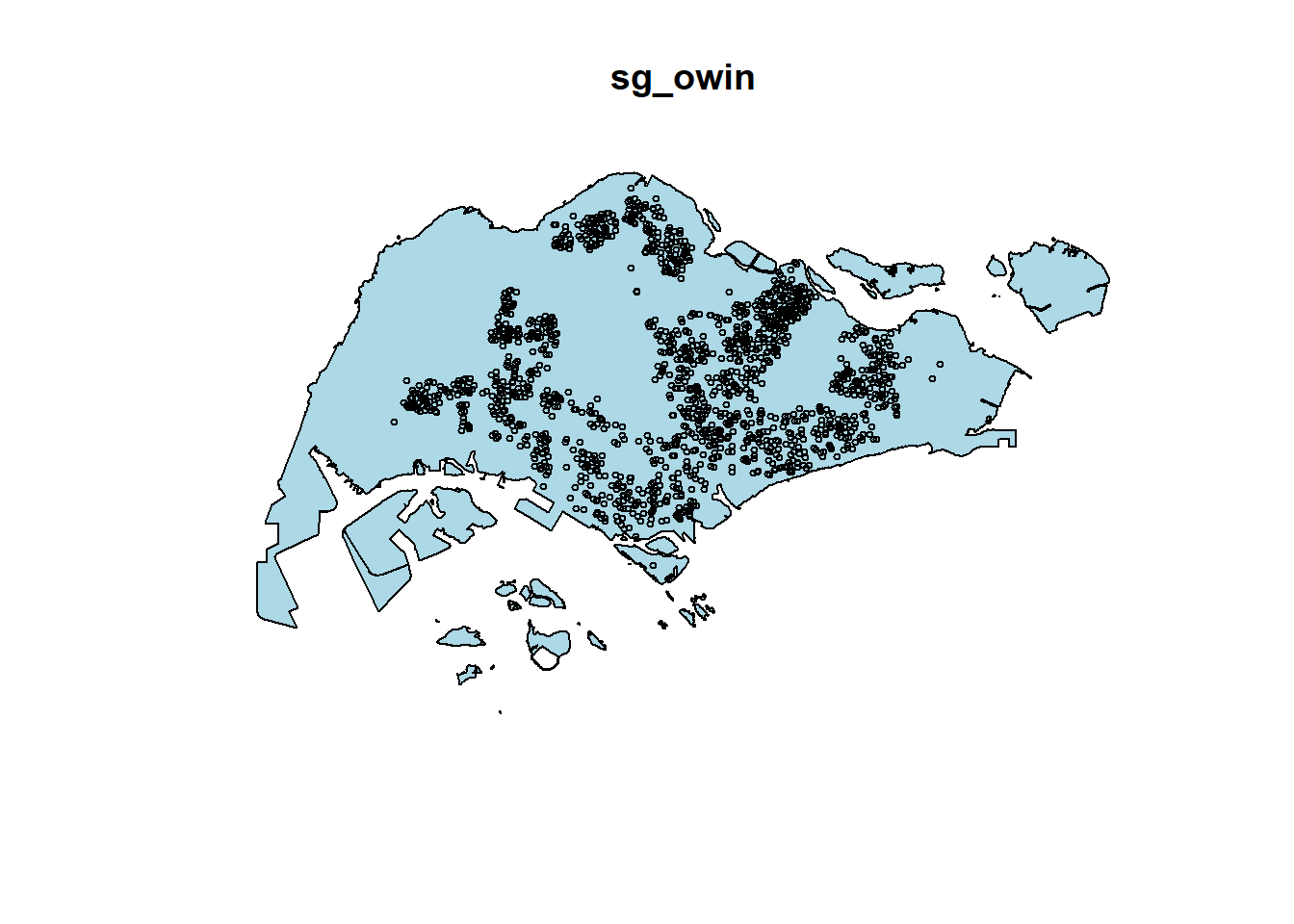
Alternative method:
plot(childcareSG_ppp)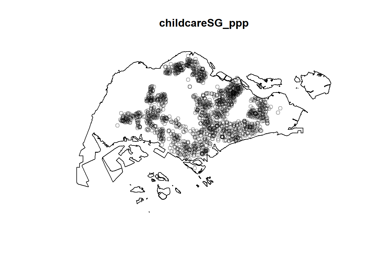
Extract study area by target planning area
pg = mpsz[mpsz@data$PLN_AREA_N == "PUNGGOL",]
tm = mpsz[mpsz@data$PLN_AREA_N == "TAMPINES",]
ck = mpsz[mpsz@data$PLN_AREA_N == "CHOA CHU KANG",]
jw = mpsz[mpsz@data$PLN_AREA_N == "JURONG WEST",]par(mfrow=c(2,2))
plot(pg, main = "Ponggol")
plot(tm, main = "Tampines")
plot(ck, main = "Choa Chu Kang")
plot(jw, main = "Jurong West")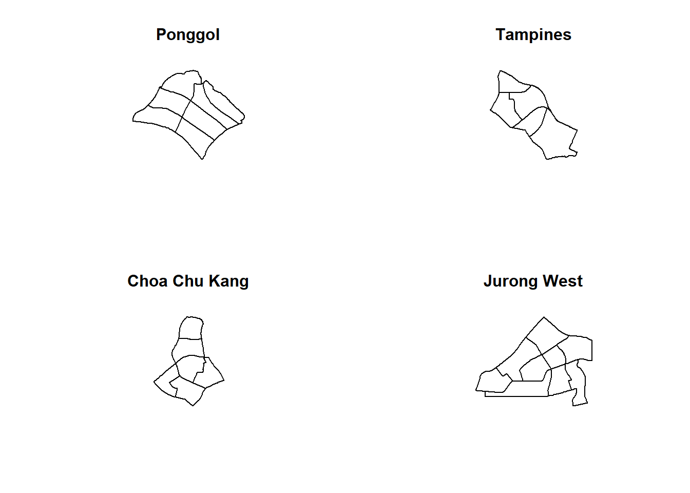
Converting spatial point data frame into generic sp format
pg_sp = as(pg, "SpatialPolygons")
tm_sp = as(tm, "SpatialPolygons")
ck_sp = as(ck, "SpatialPolygons")
jw_sp = as(jw, "SpatialPolygons")Creating owin object
pg_owin = as(pg_sp, "owin")
tm_owin = as(tm_sp, "owin")
ck_owin = as(ck_sp, "owin")
jw_owin = as(jw_sp, "owin")Combining childcare points and study areas
childcare_pg_ppp = childcare_ppp_jit[pg_owin]
childcare_tm_ppp = childcare_ppp_jit[tm_owin]
childcare_ck_ppp = childcare_ppp_jit[ck_owin]
childcare_jw_ppp = childcare_ppp_jit[jw_owin]transform the unit of measurements from m to km.
childcare_pg_ppp.km = rescale(childcare_pg_ppp, 1000, "km")
childcare_tm_ppp.km = rescale(childcare_tm_ppp, 1000, "km")
childcare_ck_ppp.km = rescale(childcare_ck_ppp, 1000, "km")
childcare_jw_ppp.km = rescale(childcare_jw_ppp, 1000, "km")Plotting them out
par(mfrow=c(2,2))
plot(childcare_pg_ppp.km, main="Punggol")
plot(childcare_tm_ppp.km, main="Tampines")
plot(childcare_ck_ppp.km, main="Choa Chu Kang")
plot(childcare_jw_ppp.km, main="Jurong West")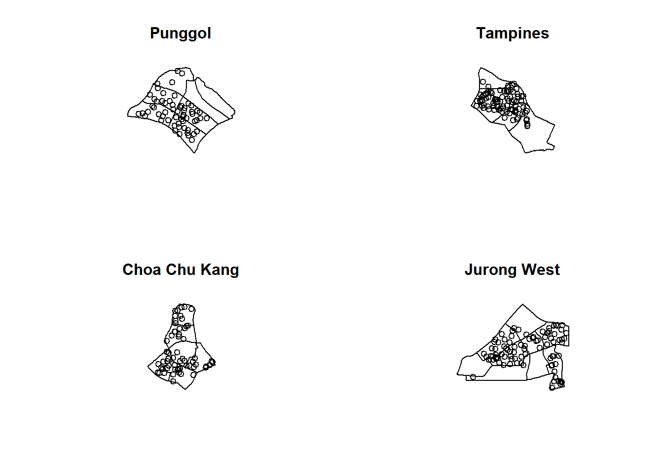
Second-order Spatial Point Pattern Analysis
Analysing spatial point process using G-function Gest() function
Estimates the nearest neighbour distance distribution function G(r) from a point pattern in a window of arbitrary shape.
The estimate of G is a useful statistic summarizing one aspect of the “clustering” points.
Choa Chu Kang Planning Area
G_CK = Gest(childcare_ck_ppp, correction = "border")
plot(G_CK, xlim=c(0,500))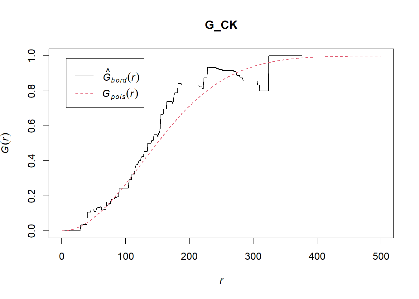
Performing complete spatial Randomness Test
Ho = The distribution of childcare services at Choa Chu Kang are randomly distributed.
H1= The distribution of childcare services at Choa Chu Kang are not randomly distributed.
The null hypothesis will be rejected if p-value is smaller than alpha value of 0.001. (99.9%)
Monte Carlo test with G-function
G_CK.csr <- envelope(childcare_ck_ppp, Gest, nsim = 999)Generating 999 simulations of CSR ...
1, 2, 3, ......10.........20.........30.........40.........50.........60........
.70.........80.........90.........100.........110.........120.........130......
...140.........150.........160.........170.........180.........190.........200....
.....210.........220.........230.........240.........250.........260.........270..
.......280.........290.........300.........310.........320.........330.........340
.........350.........360.........370.........380.........390.........400........
.410.........420.........430.........440.........450.........460.........470......
...480.........490.........500.........510.........520.........530.........540....
.....550.........560.........570.........580.........590.........600.........610..
.......620.........630.........640.........650.........660.........670.........680
.........690.........700.........710.........720.........730.........740........
.750.........760.........770.........780.........790.........800.........810......
...820.........830.........840.........850.........860.........870.........880....
.....890.........900.........910.........920.........930.........940.........950..
.......960.........970.........980.........990........ 999.
Done.plot(G_CK.csr)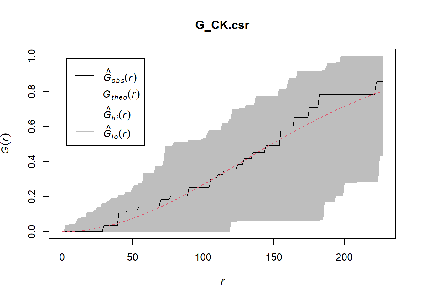
Tampines Planning Area
G_tm = Gest(childcare_tm_ppp, correction = "best")
plot(G_tm)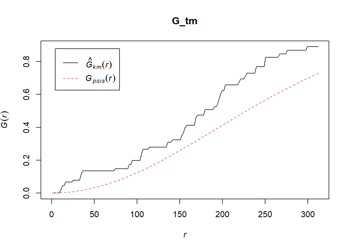
Ho = The distribution of childcare services at Tampines are randomly distributed.
H1= The distribution of childcare services at Tampines are not randomly distributed.
The null hypothesis will be rejected is p-value is smaller than alpha value of 0.001.
G_tm.csr <- envelope(childcare_tm_ppp, Gest, correction = "all", nsim = 999)Generating 999 simulations of CSR ...
1, 2, 3, ......10.........20.........30.........40.........50.........60........
.70.........80.........90.........100.........110.........120.........130......
...140.........150.........160.........170.........180.........190.........200....
.....210.........220.........230.........240.........250.........260.........270..
.......280.........290.........300.........310.........320.........330.........340
.........350.........360.........370.........380.........390.........400........
.410.........420.........430.........440.........450.........460.........470......
...480.........490.........500.........510.........520.........530.........540....
.....550.........560.........570.........580.........590.........600.........610..
.......620.........630.........640.........650.........660.........670.........680
.........690.........700.........710.........720.........730.........740........
.750.........760.........770.........780.........790.........800.........810......
...820.........830.........840.........850.........860.........870.........880....
.....890.........900.........910.........920.........930.........940.........950..
.......960.........970.........980.........990........ 999.
Done.plot(G_tm.csr)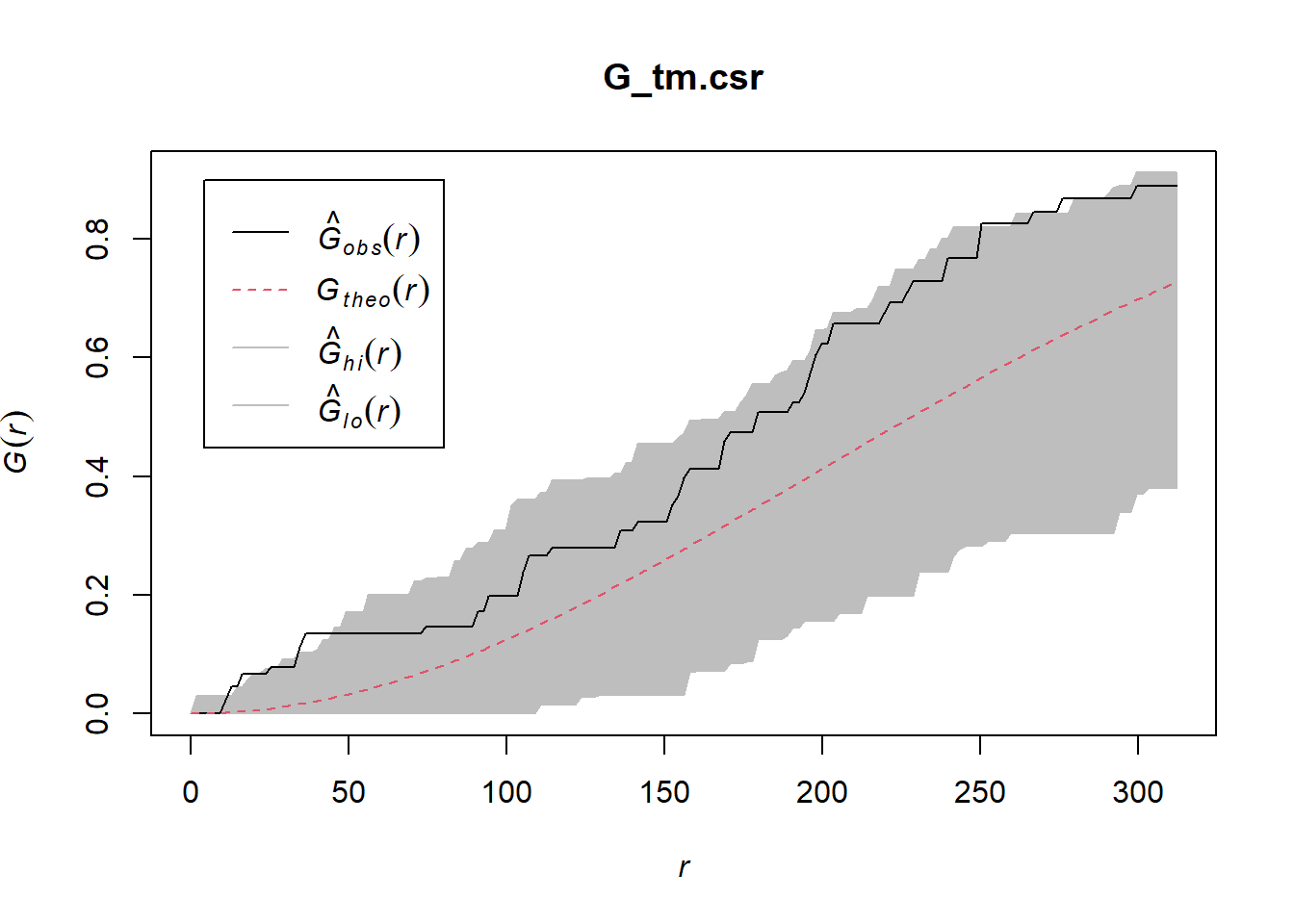
Analysing Spatial Point Process Using F-Function
Estimates the empty space function F(r) or its hazard rate h(r) from a point pattern in a window of arbitrary shape.
Choa Chu Kang Planning Area
F_CK = Fest(childcare_ck_ppp)
plot(F_CK)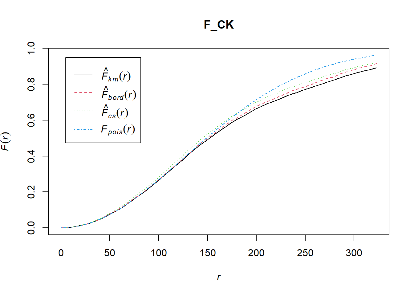
Performing Complete Spatial Randomness Test
F_CK.csr <- envelope(childcare_ck_ppp, Fest, nsim = 999)Generating 999 simulations of CSR ...
1, 2, 3, ......10.........20.........30.........40.........50.........60........
.70.........80.........90.........100.........110.........120.........130......
...140.........150.........160.........170.........180.........190.........200....
.....210.........220.........230.........240.........250.........260.........270..
.......280.........290.........300.........310.........320.........330.........340
.........350.........360.........370.........380.........390.........400........
.410.........420.........430.........440.........450.........460.........470......
...480.........490.........500.........510.........520.........530.........540....
.....550.........560.........570.........580.........590.........600.........610..
.......620.........630.........640.........650.........660.........670.........680
.........690.........700.........710.........720.........730.........740........
.750.........760.........770.........780.........790.........800.........810......
...820.........830.........840.........850.........860.........870.........880....
.....890.........900.........910.........920.........930.........940.........950..
.......960.........970.........980.........990........ 999.
Done.plot(F_CK.csr)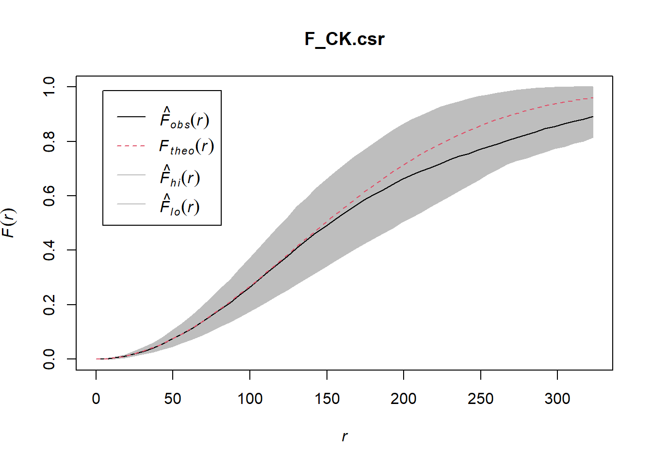
Tampines Planning Area
F_tm = Fest(childcare_tm_ppp, correction = "best")
plot(F_tm)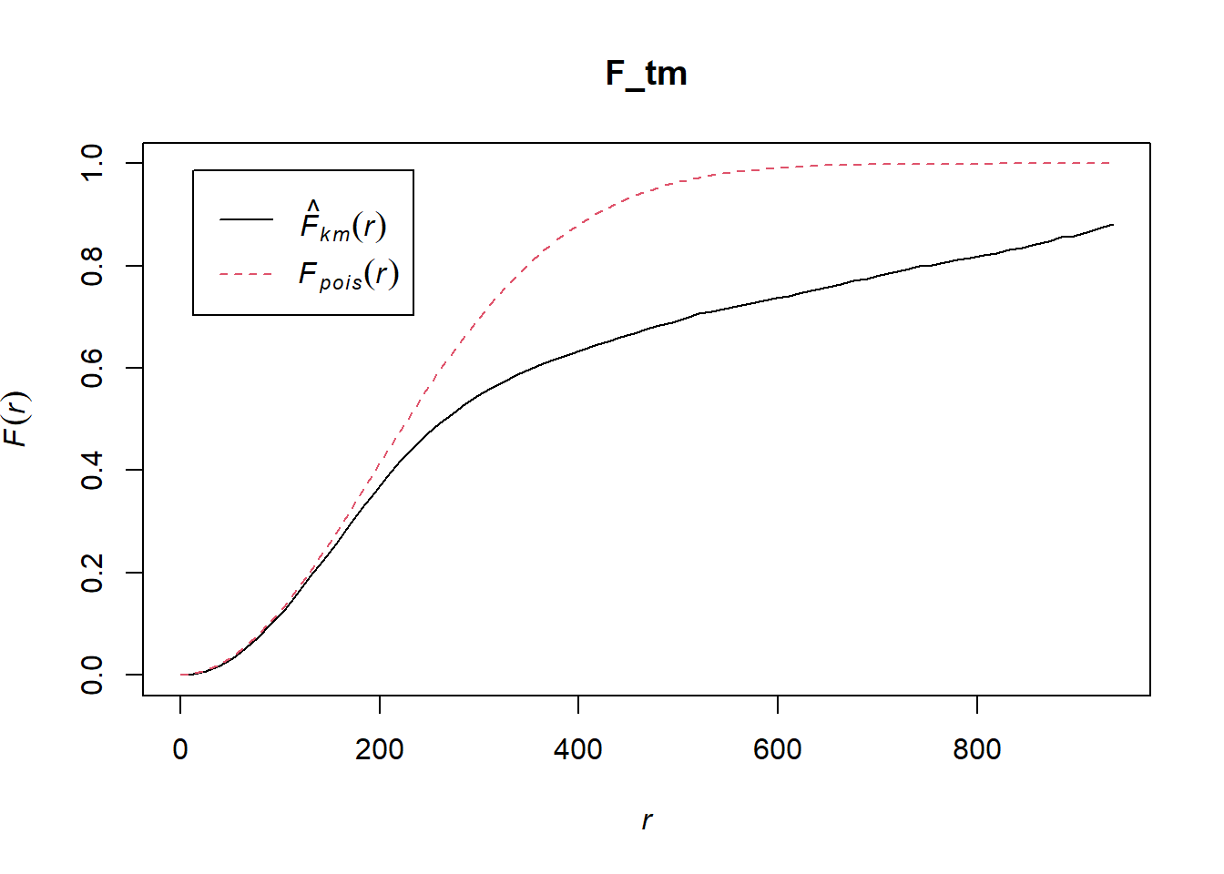
F_tm.csr <- envelope(childcare_tm_ppp, Fest, correction = "all", nsim = 999)Generating 999 simulations of CSR ...
1, 2, 3, ......10.........20.........30.........40.........50.........60........
.70.........80.........90.........100.........110.........120.........130......
...140.........150.........160.........170.........180.........190.........200....
.....210.........220.........230.........240.........250.........260.........270..
.......280.........290.........300.........310.........320.........330.........340
.........350.........360.........370.........380.........390.........400........
.410.........420.........430.........440.........450.........460.........470......
...480.........490.........500.........510.........520.........530.........540....
.....550.........560.........570.........580.........590.........600.........610..
.......620.........630.........640.........650.........660.........670.........680
.........690.........700.........710.........720.........730.........740........
.750.........760.........770.........780.........790.........800.........810......
...820.........830.........840.........850.........860.........870.........880....
.....890.........900.........910.........920.........930.........940.........950..
.......960.........970.........980.........990........ 999.
Done.plot(F_tm.csr)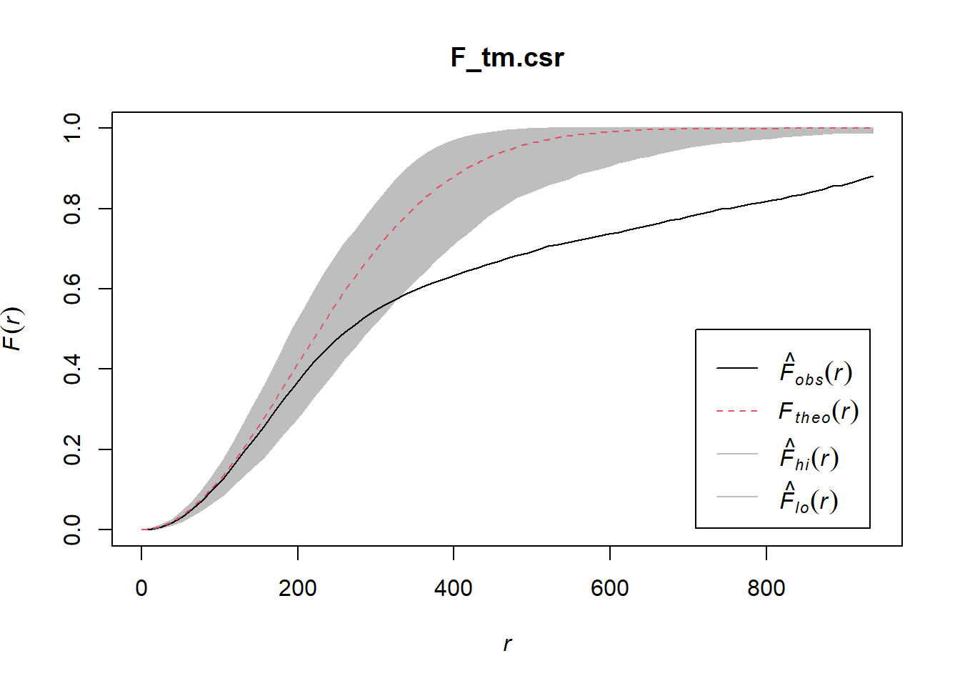
Analysing Spatial Point Process Using K-Function
K-function measures the number of events found up to a given distance of any particular event
Choa Chu Kang Planning Area
K_ck = Kest(childcare_ck_ppp, correction = "Ripley")
plot(K_ck, . -r ~ r, ylab= "K(d)-r", xlab = "d(m)")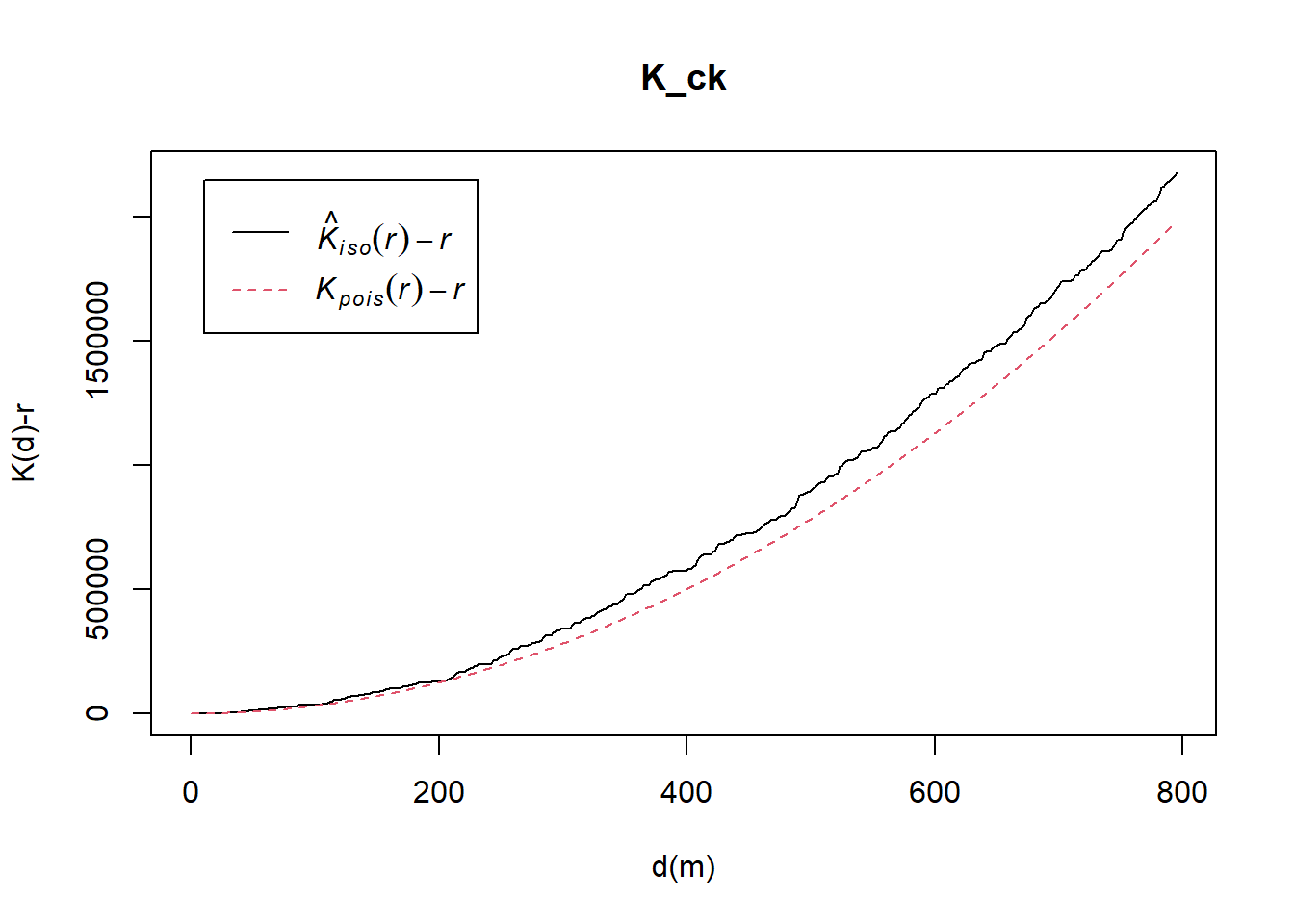
K_ck.csr <- envelope(childcare_ck_ppp, Kest, nsim = 99, rank = 1, glocal=TRUE)Generating 99 simulations of CSR ...
1, 2, 3, 4, 5, 6, 7, 8, 9, 10, 11, 12, 13, 14, 15, 16, 17, 18, 19, 20, 21, 22, 23, 24, 25, 26, 27, 28, 29, 30, 31, 32, 33, 34, 35, 36, 37, 38, 39, 40,
41, 42, 43, 44, 45, 46, 47, 48, 49, 50, 51, 52, 53, 54, 55, 56, 57, 58, 59, 60, 61, 62, 63, 64, 65, 66, 67, 68, 69, 70, 71, 72, 73, 74, 75, 76, 77, 78, 79, 80,
81, 82, 83, 84, 85, 86, 87, 88, 89, 90, 91, 92, 93, 94, 95, 96, 97, 98, 99.
Done.plot(K_ck.csr, . - r ~ r, xlab="d", ylab="K(d)-r")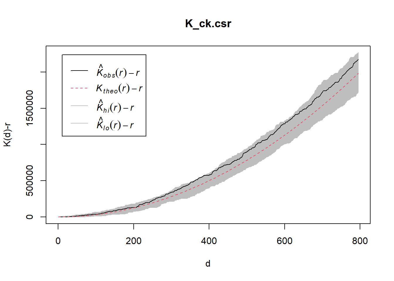
Tampines Planning Area
K_tm = Kest(childcare_tm_ppp, correction = "Ripley")
plot(K_tm, . -r ~ r,
ylab= "K(d)-r", xlab = "d(m)",
xlim=c(0,1000))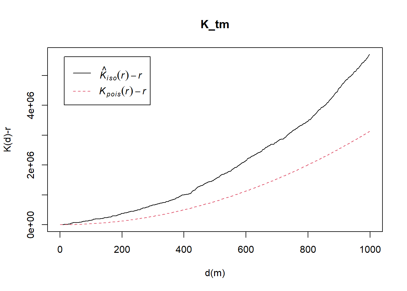
K_tm.csr <- envelope(childcare_tm_ppp, Kest, nsim = 99, rank = 1, glocal=TRUE)Generating 99 simulations of CSR ...
1, 2, 3, 4, 5, 6, 7, 8, 9, 10, 11, 12, 13, 14, 15, 16, 17, 18, 19, 20, 21, 22, 23, 24, 25, 26, 27, 28, 29, 30, 31, 32, 33, 34, 35, 36, 37, 38, 39, 40,
41, 42, 43, 44, 45, 46, 47, 48, 49, 50, 51, 52, 53, 54, 55, 56, 57, 58, 59, 60, 61, 62, 63, 64, 65, 66, 67, 68, 69, 70, 71, 72, 73, 74, 75, 76, 77, 78, 79, 80,
81, 82, 83, 84, 85, 86, 87, 88, 89, 90, 91, 92, 93, 94, 95, 96, 97, 98, 99.
Done.plot(K_tm.csr, . - r ~ r,
xlab="d", ylab="K(d)-r", xlim=c(0,500))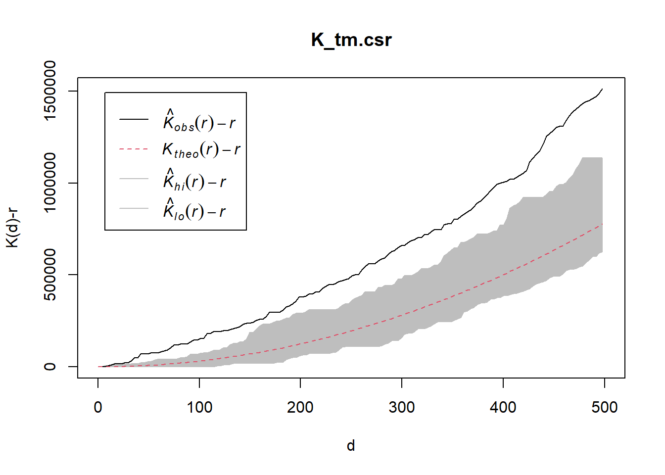
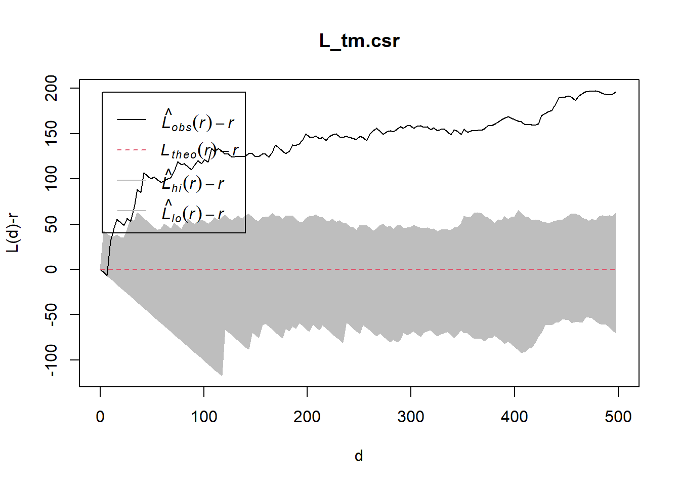
Analysing Spatial Point Process Using L-Function
Choa Chu Kang Planning Area
L_ck = Lest(childcare_ck_ppp, correction = "Ripley")
plot(L_ck, . -r ~ r,
ylab= "L(d)-r", xlab = "d(m)")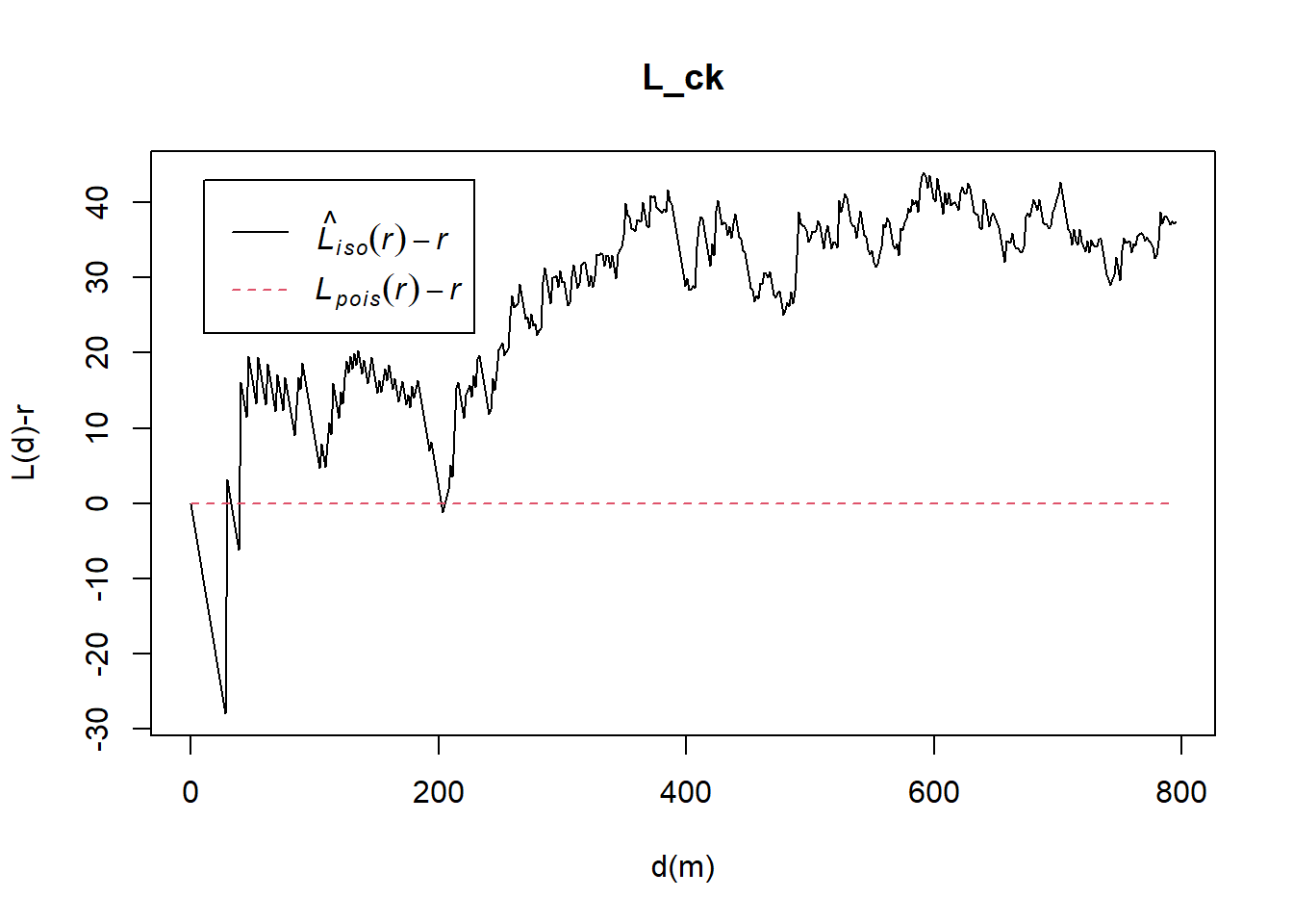
L_ck.csr <- envelope(childcare_ck_ppp, Lest, nsim = 99, rank = 1, glocal=TRUE)Generating 99 simulations of CSR ...
1, 2, 3, 4, 5, 6, 7, 8, 9, 10, 11, 12, 13, 14, 15, 16, 17, 18, 19, 20, 21, 22, 23, 24, 25, 26, 27, 28, 29, 30, 31, 32, 33, 34, 35, 36, 37, 38, 39, 40,
41, 42, 43, 44, 45, 46, 47, 48, 49, 50, 51, 52, 53, 54, 55, 56, 57, 58, 59, 60, 61, 62, 63, 64, 65, 66, 67, 68, 69, 70, 71, 72, 73, 74, 75, 76, 77, 78, 79, 80,
81, 82, 83, 84, 85, 86, 87, 88, 89, 90, 91, 92, 93, 94, 95, 96, 97, 98, 99.
Done.plot(L_ck.csr, . - r ~ r, xlab="d", ylab="L(d)-r")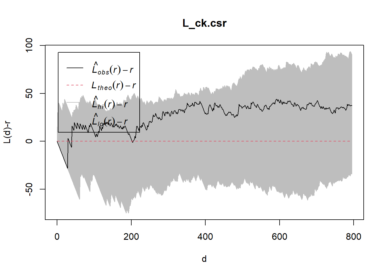
Tampines Planning Area
L_tm = Lest(childcare_tm_ppp, correction = "Ripley")
plot(L_tm, . -r ~ r,
ylab= "L(d)-r", xlab = "d(m)",
xlim=c(0,1000))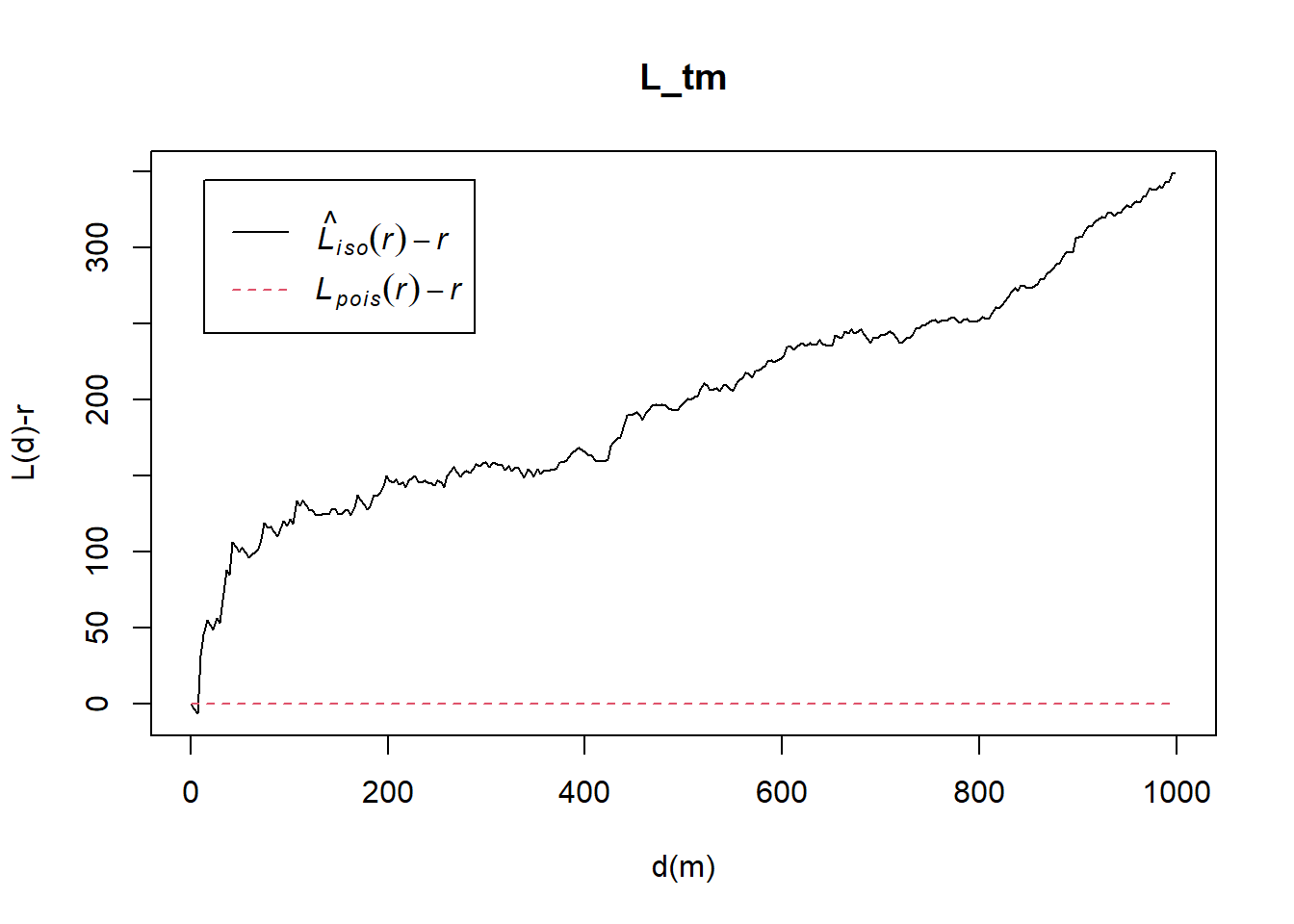
L_tm.csr <- envelope(childcare_tm_ppp, Lest, nsim = 99, rank = 1, glocal=TRUE)Generating 99 simulations of CSR ...
1, 2, 3, 4, 5, 6, 7, 8, 9, 10, 11, 12, 13, 14, 15, 16, 17, 18, 19, 20, 21, 22, 23, 24, 25, 26, 27, 28, 29, 30, 31, 32, 33, 34, 35, 36, 37, 38, 39, 40,
41, 42, 43, 44, 45, 46, 47, 48, 49, 50, 51, 52, 53, 54, 55, 56, 57, 58, 59, 60, 61, 62, 63, 64, 65, 66, 67, 68, 69, 70, 71, 72, 73, 74, 75, 76, 77, 78, 79, 80,
81, 82, 83, 84, 85, 86, 87, 88, 89, 90, 91, 92, 93, 94, 95, 96, 97, 98, 99.
Done.plot(L_tm.csr, . - r ~ r,
xlab="d", ylab="L(d)-r", xlim=c(0,500))