Hands-On Exercise 07B

Author

Xinyee How

Published

February 18, 2023

Modified

March 6, 2023

Installing packages

pacman::p_load(sf, spdep, tmap, tidyverse)

Importing geospatial data - shapefile

hunan <- st_read(dsn = "data/geospatial", 
                 layer = "Hunan")

Reading layer `Hunan' from data source 
  `C:\xinyeehow\IS415-GAA\Hands-On_Ex\Hands-On_Ex07\data\geospatial' 
  using driver `ESRI Shapefile'
Simple feature collection with 88 features and 7 fields
Geometry type: POLYGON
Dimension:     XY
Bounding box:  xmin: 108.7831 ymin: 24.6342 xmax: 114.2544 ymax: 30.12812
Geodetic CRS:  WGS 84

Importing aspatial data - csv

hunan2012 <- read_csv("data/aspatial/Hunan_2012.csv")

Performing relational join (cleaning up data)

hunan <- left_join(hunan,hunan2012) %>%
  select(1:4, 7, 15)

Visualising Regional Development Indicator

equal <- tm_shape(hunan) +
  tm_fill("GDPPC",
          n = 5,
          style = "equal") +
  tm_borders(alpha = 0.5) +
  tm_layout(main.title = "Equal interval classification")

quantile <- tm_shape(hunan) +
  tm_fill("GDPPC",
          n = 5,
          style = "quantile") +
  tm_borders(alpha = 0.5) +
  tm_layout(main.title = "Equal quantile classification")

tmap_arrange(equal, 
             quantile, 
             asp=1, 
             ncol=2)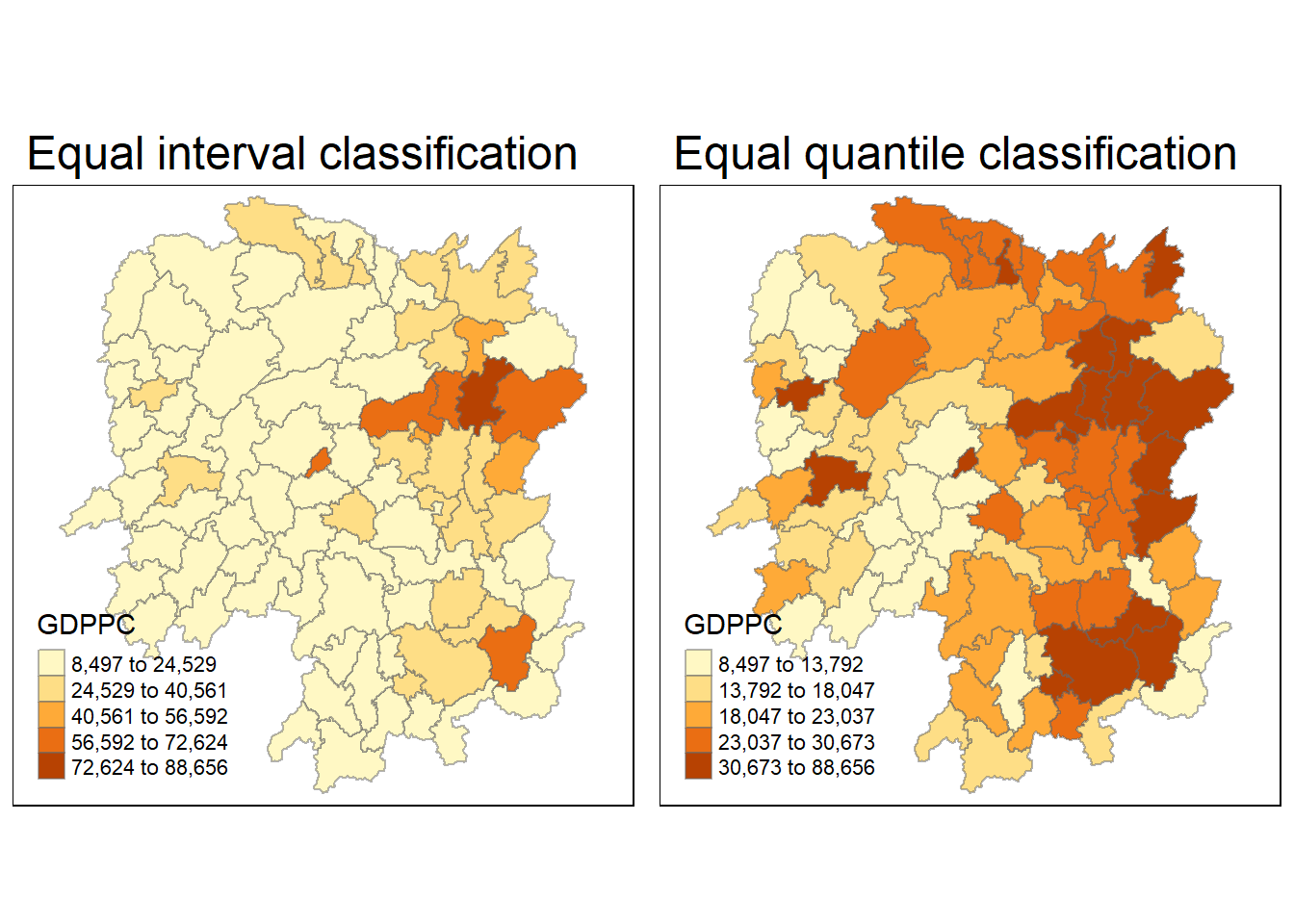

Global Spatial Autocorrelation

Computing Contiguity Spatial Weights

wm_q <- poly2nb(hunan, 
                queen=TRUE)
summary(wm_q)

Neighbour list object:
Number of regions: 88 
Number of nonzero links: 448 
Percentage nonzero weights: 5.785124 
Average number of links: 5.090909 
Link number distribution:

 1  2  3  4  5  6  7  8  9 11 
 2  2 12 16 24 14 11  4  2  1 
2 least connected regions:
30 65 with 1 link
1 most connected region:
85 with 11 links

Row-standardised weights matrix

rswm_q <- nb2listw(wm_q, 
                   style="W", 
                   zero.policy = TRUE)
rswm_q

Characteristics of weights list object:
Neighbour list object:
Number of regions: 88 
Number of nonzero links: 448 
Percentage nonzero weights: 5.785124 
Average number of links: 5.090909 

Weights style: W 
Weights constants summary:
   n   nn S0       S1       S2
W 88 7744 88 37.86334 365.9147

Global Spatial Autocorrelation: Moran’s I

Maron’s I test

moran.test(hunan$GDPPC, 
           listw=rswm_q, 
           zero.policy = TRUE, 
           na.action=na.omit)


    Moran I test under randomisation

data:  hunan$GDPPC  
weights: rswm_q    

Moran I statistic standard deviate = 4.7351, p-value = 1.095e-06
alternative hypothesis: greater
sample estimates:
Moran I statistic       Expectation          Variance 
      0.300749970      -0.011494253       0.004348351

Computing Monte Carlo Moran’s I

set.seed(1234)
bperm= moran.mc(hunan$GDPPC, 
                listw=rswm_q, 
                nsim=999, 
                zero.policy = TRUE, 
                na.action=na.omit)
bperm


    Monte-Carlo simulation of Moran I

data:  hunan$GDPPC 
weights: rswm_q  
number of simulations + 1: 1000 

statistic = 0.30075, observed rank = 1000, p-value = 0.001
alternative hypothesis: greater

Visualising Monte Carlo Moran’s I

Computing statistical values

mean(bperm$res[1:999])

[1] -0.01504572

var(bperm$res[1:999])

[1] 0.004371574

summary(bperm$res[1:999])

    Min.  1st Qu.   Median     Mean  3rd Qu.     Max. 
-0.18339 -0.06168 -0.02125 -0.01505  0.02611  0.27593

hist(bperm$res, 
     freq=TRUE, 
     breaks=20, 
     xlab="Simulated Moran's I")
abline(v=0, 
       col="red")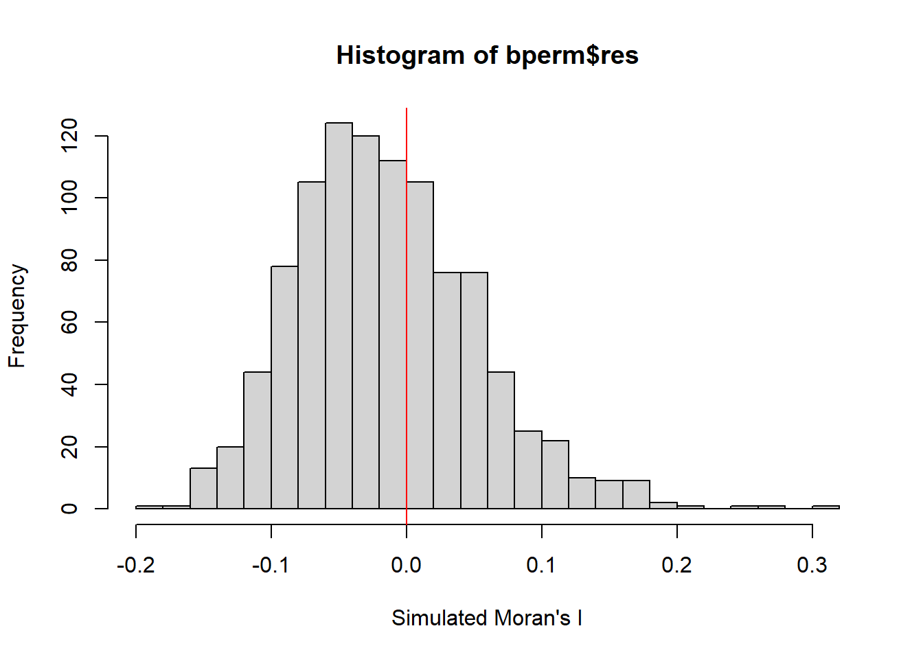

Global Spatial Autocorrelation: Geary’s

Geary’s C test

geary.test(hunan$GDPPC, listw=rswm_q)


    Geary C test under randomisation

data:  hunan$GDPPC 
weights: rswm_q 

Geary C statistic standard deviate = 3.6108, p-value = 0.0001526
alternative hypothesis: Expectation greater than statistic
sample estimates:
Geary C statistic       Expectation          Variance 
        0.6907223         1.0000000         0.0073364

Computing Monte Carlo Geary’s C

set.seed(1234)
bperm=geary.mc(hunan$GDPPC, 
               listw=rswm_q, 
               nsim=999)
bperm


    Monte-Carlo simulation of Geary C

data:  hunan$GDPPC 
weights: rswm_q 
number of simulations + 1: 1000 

statistic = 0.69072, observed rank = 1, p-value = 0.001
alternative hypothesis: greater

Visualising the Monte Carlo Geary’s C

Computing statistical values

mean(bperm$res[1:999])

[1] 1.004402

var(bperm$res[1:999])

[1] 0.007436493

summary(bperm$res[1:999])

   Min. 1st Qu.  Median    Mean 3rd Qu.    Max. 
 0.7142  0.9502  1.0052  1.0044  1.0595  1.2722

hist(bperm$res, freq=TRUE, breaks=20, xlab="Simulated Geary c")
abline(v=1, col="red")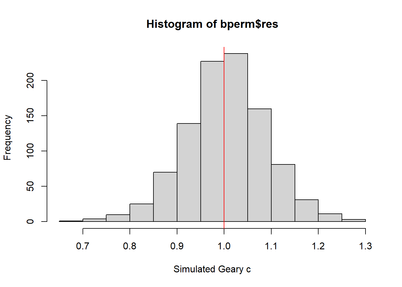

Spatial Correlogram

Compute Moran’s I correlogram

MI_corr <- sp.correlogram(wm_q, 
                          hunan$GDPPC, 
                          order=6, 
                          method="I", 
                          style="W")
plot(MI_corr)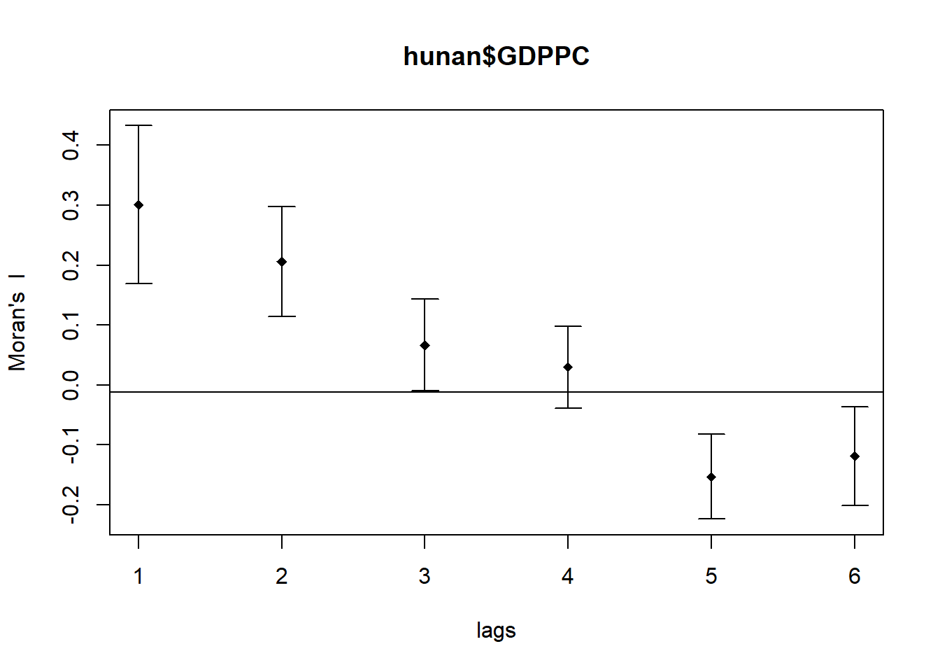

Analysis of results

print(MI_corr)

Spatial correlogram for hunan$GDPPC 
method: Moran's I
         estimate expectation   variance standard deviate Pr(I) two sided    
1 (88)  0.3007500  -0.0114943  0.0043484           4.7351       2.189e-06 ***
2 (88)  0.2060084  -0.0114943  0.0020962           4.7505       2.029e-06 ***
3 (88)  0.0668273  -0.0114943  0.0014602           2.0496        0.040400 *  
4 (88)  0.0299470  -0.0114943  0.0011717           1.2107        0.226015    
5 (88) -0.1530471  -0.0114943  0.0012440          -4.0134       5.984e-05 ***
6 (88) -0.1187070  -0.0114943  0.0016791          -2.6164        0.008886 ** 
---
Signif. codes:  0 '***' 0.001 '**' 0.01 '*' 0.05 '.' 0.1 ' ' 1

Compute Geary’s C correlogram and plot

GC_corr <- sp.correlogram(wm_q, 
                          hunan$GDPPC, 
                          order=6, 
                          method="C", 
                          style="W")
plot(GC_corr)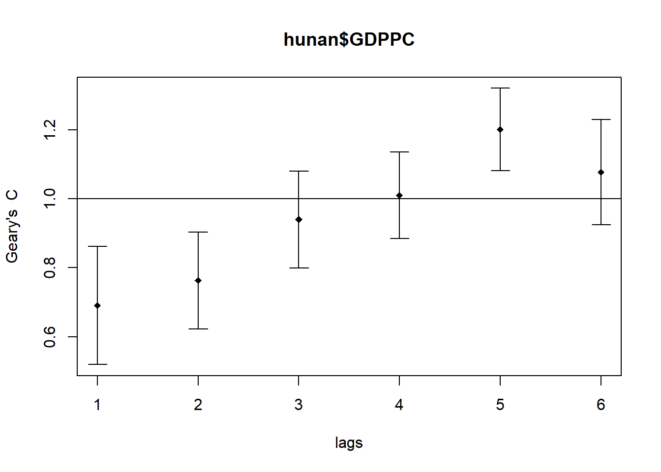

Analysis of results

print(GC_corr)

Spatial correlogram for hunan$GDPPC 
method: Geary's C
        estimate expectation  variance standard deviate Pr(I) two sided    
1 (88) 0.6907223   1.0000000 0.0073364          -3.6108       0.0003052 ***
2 (88) 0.7630197   1.0000000 0.0049126          -3.3811       0.0007220 ***
3 (88) 0.9397299   1.0000000 0.0049005          -0.8610       0.3892612    
4 (88) 1.0098462   1.0000000 0.0039631           0.1564       0.8757128    
5 (88) 1.2008204   1.0000000 0.0035568           3.3673       0.0007592 ***
6 (88) 1.0773386   1.0000000 0.0058042           1.0151       0.3100407    
---
Signif. codes:  0 '***' 0.001 '**' 0.01 '*' 0.05 '.' 0.1 ' ' 1

Cluster and Outlier Analysis

Computing local Moran’s I

fips <- order(hunan$County)
localMI <- localmoran(hunan$GDPPC, rswm_q)
head(localMI)

            Ii          E.Ii       Var.Ii        Z.Ii Pr(z != E(Ii))
1 -0.001468468 -2.815006e-05 4.723841e-04 -0.06626904      0.9471636
2  0.025878173 -6.061953e-04 1.016664e-02  0.26266425      0.7928094
3 -0.011987646 -5.366648e-03 1.133362e-01 -0.01966705      0.9843090
4  0.001022468 -2.404783e-07 5.105969e-06  0.45259801      0.6508382
5  0.014814881 -6.829362e-05 1.449949e-03  0.39085814      0.6959021
6 -0.038793829 -3.860263e-04 6.475559e-03 -0.47728835      0.6331568

Local Moran matrix

printCoefmat(data.frame(
  localMI[fips,], 
  row.names=hunan$County[fips]),
  check.names=FALSE)

                       Ii        E.Ii      Var.Ii        Z.Ii Pr.z....E.Ii..
Anhua         -2.2493e-02 -5.0048e-03  5.8235e-02 -7.2467e-02         0.9422
Anren         -3.9932e-01 -7.0111e-03  7.0348e-02 -1.4791e+00         0.1391
Anxiang       -1.4685e-03 -2.8150e-05  4.7238e-04 -6.6269e-02         0.9472
Baojing        3.4737e-01 -5.0089e-03  8.3636e-02  1.2185e+00         0.2230
Chaling        2.0559e-02 -9.6812e-04  2.7711e-02  1.2932e-01         0.8971
Changning     -2.9868e-05 -9.0010e-09  1.5105e-07 -7.6828e-02         0.9388
Changsha       4.9022e+00 -2.1348e-01  2.3194e+00  3.3590e+00         0.0008
Chengbu        7.3725e-01 -1.0534e-02  2.2132e-01  1.5895e+00         0.1119
Chenxi         1.4544e-01 -2.8156e-03  4.7116e-02  6.8299e-01         0.4946
Cili           7.3176e-02 -1.6747e-03  4.7902e-02  3.4200e-01         0.7324
Dao            2.1420e-01 -2.0824e-03  4.4123e-02  1.0297e+00         0.3032
Dongan         1.5210e-01 -6.3485e-04  1.3471e-02  1.3159e+00         0.1882
Dongkou        5.2918e-01 -6.4461e-03  1.0748e-01  1.6338e+00         0.1023
Fenghuang      1.8013e-01 -6.2832e-03  1.3257e-01  5.1198e-01         0.6087
Guidong       -5.9160e-01 -1.3086e-02  3.7003e-01 -9.5104e-01         0.3416
Guiyang        1.8240e-01 -3.6908e-03  3.2610e-02  1.0305e+00         0.3028
Guzhang        2.8466e-01 -8.5054e-03  1.4152e-01  7.7931e-01         0.4358
Hanshou        2.5878e-02 -6.0620e-04  1.0167e-02  2.6266e-01         0.7928
Hengdong       9.9964e-03 -4.9063e-04  6.7742e-03  1.2742e-01         0.8986
Hengnan        2.8064e-02 -3.2160e-04  3.7597e-03  4.6294e-01         0.6434
Hengshan      -5.8201e-03 -3.0437e-05  5.1076e-04 -2.5618e-01         0.7978
Hengyang       6.2997e-02 -1.3046e-03  2.1865e-02  4.3486e-01         0.6637
Hongjiang      1.8790e-01 -2.3019e-03  3.1725e-02  1.0678e+00         0.2856
Huarong       -1.5389e-02 -1.8667e-03  8.1030e-02 -4.7503e-02         0.9621
Huayuan        8.3772e-02 -8.5569e-04  2.4495e-02  5.4072e-01         0.5887
Huitong        2.5997e-01 -5.2447e-03  1.1077e-01  7.9685e-01         0.4255
Jiahe         -1.2431e-01 -3.0550e-03  5.1111e-02 -5.3633e-01         0.5917
Jianghua       2.8651e-01 -3.8280e-03  8.0968e-02  1.0204e+00         0.3076
Jiangyong      2.4337e-01 -2.7082e-03  1.1746e-01  7.1800e-01         0.4728
Jingzhou       1.8270e-01 -8.5106e-04  2.4363e-02  1.1759e+00         0.2396
Jinshi        -1.1988e-02 -5.3666e-03  1.1334e-01 -1.9667e-02         0.9843
Jishou        -2.8680e-01 -2.6305e-03  4.4028e-02 -1.3543e+00         0.1756
Lanshan        6.3334e-02 -9.6365e-04  2.0441e-02  4.4972e-01         0.6529
Leiyang        1.1581e-02 -1.4948e-04  2.5082e-03  2.3422e-01         0.8148
Lengshuijiang -1.7903e+00 -8.2129e-02  2.1598e+00 -1.1623e+00         0.2451
Li             1.0225e-03 -2.4048e-07  5.1060e-06  4.5260e-01         0.6508
Lianyuan      -1.4672e-01 -1.8983e-03  1.9145e-02 -1.0467e+00         0.2952
Liling         1.3774e+00 -1.5097e-02  4.2601e-01  2.1335e+00         0.0329
Linli          1.4815e-02 -6.8294e-05  1.4499e-03  3.9086e-01         0.6959
Linwu         -2.4621e-03 -9.0703e-06  1.9258e-04 -1.7676e-01         0.8597
Linxiang       6.5904e-02 -2.9028e-03  2.5470e-01  1.3634e-01         0.8916
Liuyang        3.3688e+00 -7.7502e-02  1.5180e+00  2.7972e+00         0.0052
Longhui        8.0801e-01 -1.1377e-02  1.5538e-01  2.0787e+00         0.0376
Longshan       7.5663e-01 -1.1100e-02  3.1449e-01  1.3690e+00         0.1710
Luxi           1.8177e-01 -2.4855e-03  3.4249e-02  9.9561e-01         0.3194
Mayang         2.1852e-01 -5.8773e-03  9.8049e-02  7.1663e-01         0.4736
Miluo          1.8704e+00 -1.6927e-02  2.7925e-01  3.5715e+00         0.0004
Nan           -9.5789e-03 -4.9497e-04  6.8341e-03 -1.0988e-01         0.9125
Ningxiang      1.5607e+00 -7.3878e-02  8.0012e-01  1.8274e+00         0.0676
Ningyuan       2.0910e-01 -7.0884e-03  8.2306e-02  7.5356e-01         0.4511
Pingjiang     -9.8964e-01 -2.6457e-03  5.6027e-02 -4.1698e+00         0.0000
Qidong         1.1806e-01 -2.1207e-03  2.4747e-02  7.6396e-01         0.4449
Qiyang         6.1966e-02 -7.3374e-04  8.5743e-03  6.7712e-01         0.4983
Rucheng       -3.6992e-01 -8.8999e-03  2.5272e-01 -7.1814e-01         0.4727
Sangzhi        2.5053e-01 -4.9470e-03  6.8000e-02  9.7972e-01         0.3272
Shaodong      -3.2659e-02 -3.6592e-05  5.0546e-04 -1.4510e+00         0.1468
Shaoshan       2.1223e+00 -5.0227e-02  1.3668e+00  1.8583e+00         0.0631
Shaoyang       5.9499e-01 -1.1253e-02  1.3012e-01  1.6807e+00         0.0928
Shimen        -3.8794e-02 -3.8603e-04  6.4756e-03 -4.7729e-01         0.6332
Shuangfeng     9.2835e-03 -2.2867e-03  3.1516e-02  6.5174e-02         0.9480
Shuangpai      8.0591e-02 -3.1366e-04  8.9838e-03  8.5358e-01         0.3933
Suining        3.7585e-01 -3.5933e-03  4.1870e-02  1.8544e+00         0.0637
Taojiang      -2.5394e-01 -1.2395e-03  1.4477e-02 -2.1002e+00         0.0357
Taoyuan        1.4729e-02 -1.2039e-04  8.5103e-04  5.0903e-01         0.6107
Tongdao        4.6482e-01 -6.9870e-03  1.9879e-01  1.0582e+00         0.2900
Wangcheng      4.4220e+00 -1.1067e-01  1.3596e+00  3.8873e+00         0.0001
Wugang         7.1003e-01 -7.8144e-03  1.0710e-01  2.1935e+00         0.0283
Xiangtan       2.4530e-01 -3.6457e-04  3.2319e-03  4.3213e+00         0.0000
Xiangxiang     2.6271e-01 -1.2703e-03  2.1290e-02  1.8092e+00         0.0704
Xiangyin       5.4525e-01 -4.7442e-03  7.9236e-02  1.9539e+00         0.0507
Xinhua         1.1810e-01 -6.2649e-03  8.6001e-02  4.2409e-01         0.6715
Xinhuang       1.5725e-01 -4.1820e-03  3.6648e-01  2.6667e-01         0.7897
Xinning        6.8928e-01 -9.6674e-03  2.0328e-01  1.5502e+00         0.1211
Xinshao        5.7578e-02 -8.5932e-03  1.1769e-01  1.9289e-01         0.8470
Xintian       -7.4050e-03 -5.1493e-03  1.0877e-01 -6.8395e-03         0.9945
Xupu           3.2406e-01 -5.7468e-03  5.7735e-02  1.3726e+00         0.1699
Yanling       -6.9021e-02 -5.9211e-04  9.9306e-03 -6.8667e-01         0.4923
Yizhang       -2.6844e-01 -2.2463e-03  4.7588e-02 -1.2202e+00         0.2224
Yongshun       6.3064e-01 -1.1350e-02  1.8830e-01  1.4795e+00         0.1390
Yongxing       4.3411e-01 -9.0735e-03  1.5088e-01  1.1409e+00         0.2539
You            7.8750e-02 -7.2728e-03  1.2116e-01  2.4714e-01         0.8048
Yuanjiang      2.0004e-04 -1.7760e-04  2.9798e-03  6.9181e-03         0.9945
Yuanling       8.7298e-03 -2.2981e-06  2.3221e-05  1.8121e+00         0.0700
Yueyang        4.1189e-02 -1.9768e-04  2.3113e-03  8.6085e-01         0.3893
Zhijiang       1.0476e-01 -7.8123e-04  1.3100e-02  9.2214e-01         0.3565
Zhongfang     -2.2685e-01 -2.1455e-03  3.5927e-02 -1.1855e+00         0.2358
Zhuzhou        3.2864e-01 -5.2432e-04  7.2391e-03  3.8688e+00         0.0001
Zixing        -7.6849e-01 -8.8210e-02  9.4057e-01 -7.0144e-01         0.4830

Mapping the local Moran’s I

hunan.localMI <- cbind(hunan,localMI) %>%
  rename(Pr.Ii = Pr.z....E.Ii..)

Mapping local Moran’s I values

tm_shape(hunan.localMI) +
  tm_fill(col = "Ii", 
          style = "pretty",
          palette = "RdBu",
          title = "local moran statistics") +
  tm_borders(alpha = 0.5)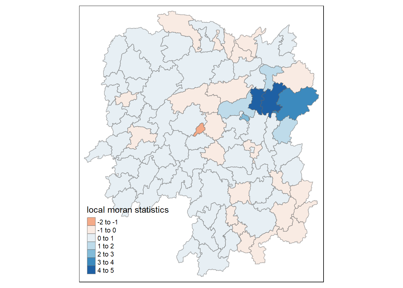

Mapping local Moran’s I p-values

tm_shape(hunan.localMI) +
  tm_fill(col = "Pr.Ii", 
          breaks=c(-Inf, 0.001, 0.01, 0.05, 0.1, Inf),
          palette="-Blues", 
          title = "local Moran's I p-values") +
  tm_borders(alpha = 0.5)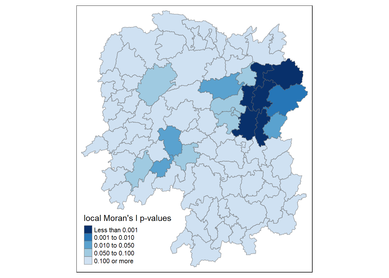

Mapping both local Moran’s I values and p-values

localMI.map <- tm_shape(hunan.localMI) +
  tm_fill(col = "Ii", 
          style = "pretty", 
          title = "local moran statistics") +
  tm_borders(alpha = 0.5)

pvalue.map <- tm_shape(hunan.localMI) +
  tm_fill(col = "Pr.Ii", 
          breaks=c(-Inf, 0.001, 0.01, 0.05, 0.1, Inf),
          palette="-Blues", 
          title = "local Moran's I p-values") +
  tm_borders(alpha = 0.5)

tmap_arrange(localMI.map, pvalue.map, asp=1, ncol=2)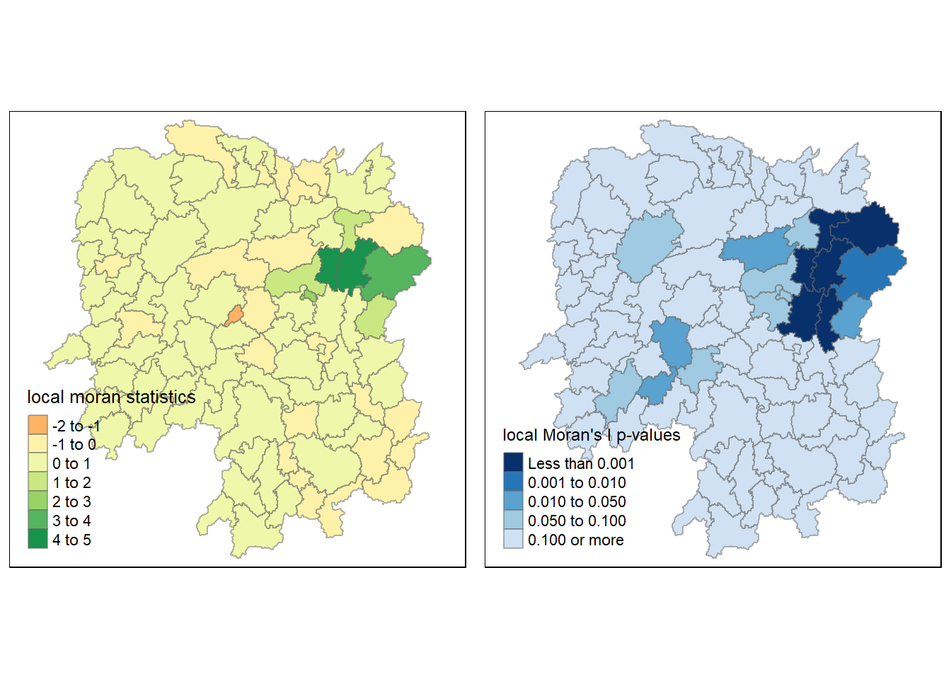

Creating a LISA Cluster Map

Plotting Moran scatterplot

nci <- moran.plot(hunan$GDPPC, rswm_q,
                  labels=as.character(hunan$County), 
                  xlab="GDPPC 2012", 
                  ylab="Spatially Lag GDPPC 2012")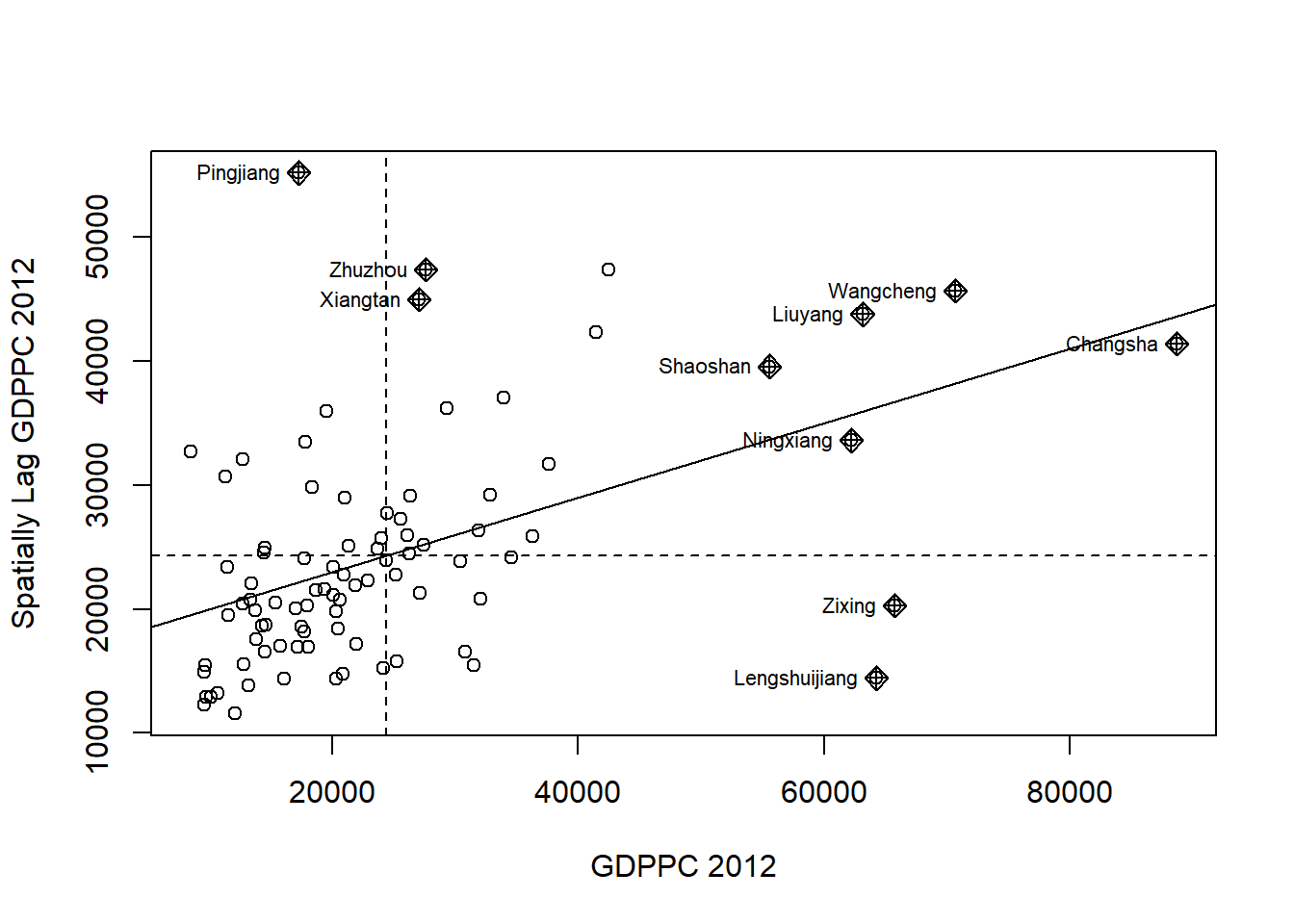

Plotting Moran scatterplot with standardised variable

Scaling and converting to vector

hunan$Z.GDPPC <- scale(hunan$GDPPC) %>% 
  as.vector

Plotting graph

nci2 <- moran.plot(hunan$Z.GDPPC, rswm_q,
                   labels=as.character(hunan$County),
                   xlab="z-GDPPC 2012", 
                   ylab="Spatially Lag z-GDPPC 2012")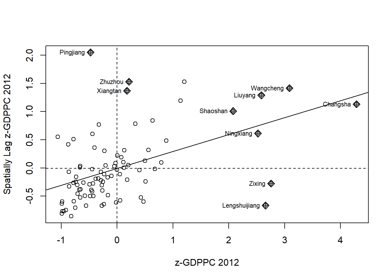

Preparing LISA map classes

Preparing LISA cluster map

quadrant <- vector(mode="numeric",length=nrow(localMI))

Derive the spatially lagged variable of interest (i.e. GDPPC) and center the spatially lagged variable around its mean

hunan$lag_GDPPC <- lag.listw(rswm_q, hunan$GDPPC)
DV <- hunan$lag_GDPPC - mean(hunan$lag_GDPPC)

Centering the local Moran’s around the mean

LM_I <- localMI[,1] - mean(localMI[,1])

Setting significance level

signif <- 0.05

Defining the low-low (1), low-high (2), high-low (3) and high-high (4) categories

quadrant[DV <0 & LM_I>0] <- 1
quadrant[DV >0 & LM_I<0] <- 2
quadrant[DV <0 & LM_I<0] <- 3  
quadrant[DV >0 & LM_I>0] <- 4

Place non-significant Moran in the category 0

quadrant[localMI[,5]>signif] <- 0

ALTERNATIVE: combining all steps into one chunk

quadrant <- vector(mode="numeric",length=nrow(localMI))
hunan$lag_GDPPC <- lag.listw(rswm_q, hunan$GDPPC)
DV <- hunan$lag_GDPPC - mean(hunan$lag_GDPPC)     
LM_I <- localMI[,1]   
signif <- 0.05       
quadrant[DV <0 & LM_I>0] <- 1
quadrant[DV >0 & LM_I<0] <- 2
quadrant[DV <0 & LM_I<0] <- 3  
quadrant[DV >0 & LM_I>0] <- 4    
quadrant[localMI[,5]>signif] <- 0

Plotting LISA map

hunan.localMI$quadrant <- quadrant
colors <- c("#ffffff", "#2c7bb6", "#abd9e9", "#fdae61", "#d7191c")
clusters <- c("insignificant", "low-low", "low-high", "high-low", "high-high")

tm_shape(hunan.localMI) +
  tm_fill(col = "quadrant", 
          style = "cat", 
          palette = colors[c(sort(unique(quadrant)))+1], 
          labels = clusters[c(sort(unique(quadrant)))+1],
          popup.vars = c("")) +
  tm_view(set.zoom.limits = c(11,17)) +
  tm_borders(alpha=0.5)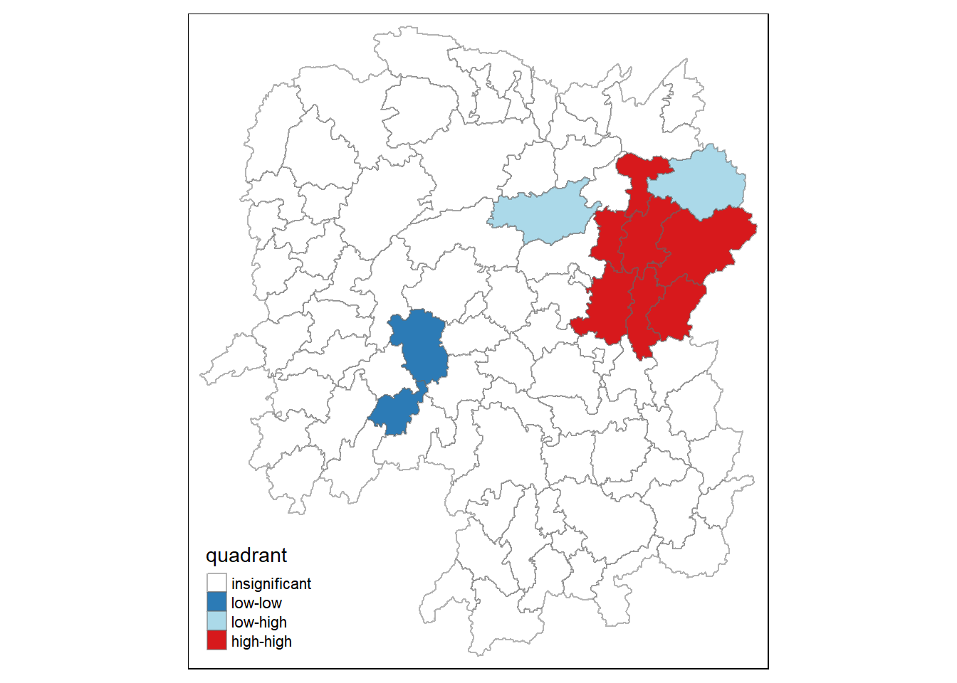

Plotting both the local Moran’s I values map and its corresponding p-values map next to each other

gdppc <- qtm(hunan, "GDPPC")

hunan.localMI$quadrant <- quadrant
colors <- c("#ffffff", "#2c7bb6", "#abd9e9", "#fdae61", "#d7191c")
clusters <- c("insignificant", "low-low", "low-high", "high-low", "high-high")

LISAmap <- tm_shape(hunan.localMI) +
  tm_fill(col = "quadrant", 
          style = "cat", 
          palette = colors[c(sort(unique(quadrant)))+1], 
          labels = clusters[c(sort(unique(quadrant)))+1],
          popup.vars = c("")) +
  tm_view(set.zoom.limits = c(11,17)) +
  tm_borders(alpha=0.5)

tmap_arrange(gdppc, LISAmap, 
             asp=1, ncol=2)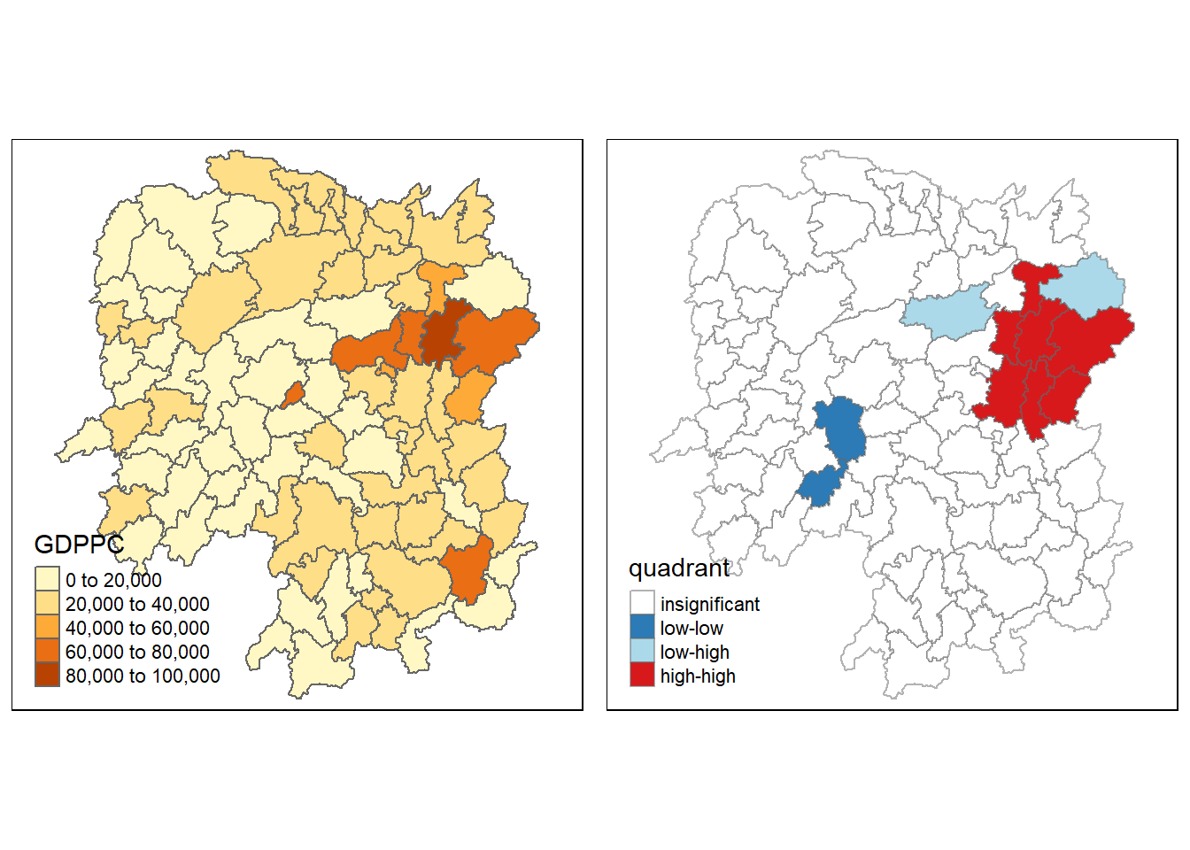

Hot Spot and Cold Spot Area Analysis

Deriving distance-based weight matrix

Deriving the centroid

longitude <- map_dbl(hunan$geometry, ~st_centroid(.x)[[1]])

latitude <- map_dbl(hunan$geometry, ~st_centroid(.x)[[2]])

coords <- cbind(longitude, latitude)

Determining the cut-off distance

#coords <- coordinates(hunan)
k1 <- knn2nb(knearneigh(coords))
k1dists <- unlist(nbdists(k1, coords, longlat = TRUE))
summary(k1dists)

   Min. 1st Qu.  Median    Mean 3rd Qu.    Max. 
  24.79   32.57   38.01   39.07   44.52   61.79

Computing fixed distance weight matrix

wm_d62 <- dnearneigh(coords, 0, 62, longlat = TRUE)
wm_d62

Neighbour list object:
Number of regions: 88 
Number of nonzero links: 324 
Percentage nonzero weights: 4.183884 
Average number of links: 3.681818

Converting the nb object into spatial weights object

wm62_lw <- nb2listw(wm_d62, style = 'B')
summary(wm62_lw)

Characteristics of weights list object:
Neighbour list object:
Number of regions: 88 
Number of nonzero links: 324 
Percentage nonzero weights: 4.183884 
Average number of links: 3.681818 
Link number distribution:

 1  2  3  4  5  6 
 6 15 14 26 20  7 
6 least connected regions:
6 15 30 32 56 65 with 1 link
7 most connected regions:
21 28 35 45 50 52 82 with 6 links

Weights style: B 
Weights constants summary:
   n   nn  S0  S1   S2
B 88 7744 324 648 5440

Computing adaptive distance weight matrix

knn <- knn2nb(knearneigh(coords, k=8))
knn

Neighbour list object:
Number of regions: 88 
Number of nonzero links: 704 
Percentage nonzero weights: 9.090909 
Average number of links: 8 
Non-symmetric neighbours list

Converting the nb object into spatial weights object

knn_lw <- nb2listw(knn, style = 'B')
summary(knn_lw)

Characteristics of weights list object:
Neighbour list object:
Number of regions: 88 
Number of nonzero links: 704 
Percentage nonzero weights: 9.090909 
Average number of links: 8 
Non-symmetric neighbours list
Link number distribution:

 8 
88 
88 least connected regions:
1 2 3 4 5 6 7 8 9 10 11 12 13 14 15 16 17 18 19 20 21 22 23 24 25 26 27 28 29 30 31 32 33 34 35 36 37 38 39 40 41 42 43 44 45 46 47 48 49 50 51 52 53 54 55 56 57 58 59 60 61 62 63 64 65 66 67 68 69 70 71 72 73 74 75 76 77 78 79 80 81 82 83 84 85 86 87 88 with 8 links
88 most connected regions:
1 2 3 4 5 6 7 8 9 10 11 12 13 14 15 16 17 18 19 20 21 22 23 24 25 26 27 28 29 30 31 32 33 34 35 36 37 38 39 40 41 42 43 44 45 46 47 48 49 50 51 52 53 54 55 56 57 58 59 60 61 62 63 64 65 66 67 68 69 70 71 72 73 74 75 76 77 78 79 80 81 82 83 84 85 86 87 88 with 8 links

Weights style: B 
Weights constants summary:
   n   nn  S0   S1    S2
B 88 7744 704 1300 23014

Computing Gi statistics

Gi statistics using fixed distance

fips <- order(hunan$County)
gi.fixed <- localG(hunan$GDPPC, wm62_lw)
gi.fixed

 [1]  0.436075843 -0.265505650 -0.073033665  0.413017033  0.273070579
 [6] -0.377510776  2.863898821  2.794350420  5.216125401  0.228236603
[11]  0.951035346 -0.536334231  0.176761556  1.195564020 -0.033020610
[16]  1.378081093 -0.585756761 -0.419680565  0.258805141  0.012056111
[21] -0.145716531 -0.027158687 -0.318615290 -0.748946051 -0.961700582
[26] -0.796851342 -1.033949773 -0.460979158 -0.885240161 -0.266671512
[31] -0.886168613 -0.855476971 -0.922143185 -1.162328599  0.735582222
[36] -0.003358489 -0.967459309 -1.259299080 -1.452256513 -1.540671121
[41] -1.395011407 -1.681505286 -1.314110709 -0.767944457 -0.192889342
[46]  2.720804542  1.809191360 -1.218469473 -0.511984469 -0.834546363
[51] -0.908179070 -1.541081516 -1.192199867 -1.075080164 -1.631075961
[56] -0.743472246  0.418842387  0.832943753 -0.710289083 -0.449718820
[61] -0.493238743 -1.083386776  0.042979051  0.008596093  0.136337469
[66]  2.203411744  2.690329952  4.453703219 -0.340842743 -0.129318589
[71]  0.737806634 -1.246912658  0.666667559  1.088613505 -0.985792573
[76]  1.233609606 -0.487196415  1.626174042 -1.060416797  0.425361422
[81] -0.837897118 -0.314565243  0.371456331  4.424392623 -0.109566928
[86]  1.364597995 -1.029658605 -0.718000620
attr(,"cluster")
 [1] Low  Low  High High High High High High High Low  Low  High Low  Low  Low 
[16] High High High High Low  High High Low  Low  High Low  Low  Low  Low  Low 
[31] Low  Low  Low  High Low  Low  Low  Low  Low  Low  High Low  Low  Low  Low 
[46] High High Low  Low  Low  Low  High Low  Low  Low  Low  Low  High Low  Low 
[61] Low  Low  Low  High High High Low  High Low  Low  High Low  High High Low 
[76] High Low  Low  Low  Low  Low  Low  High High Low  High Low  Low 
Levels: Low High
attr(,"gstari")
[1] FALSE
attr(,"call")
localG(x = hunan$GDPPC, listw = wm62_lw)
attr(,"class")
[1] "localG"

Joining the Gi values to their corresponding hunan sf data frame

hunan.gi <- cbind(hunan, as.matrix(gi.fixed)) %>%
  rename(gstat_fixed = as.matrix.gi.fixed.)

Mapping Gi values with fixed distance weights

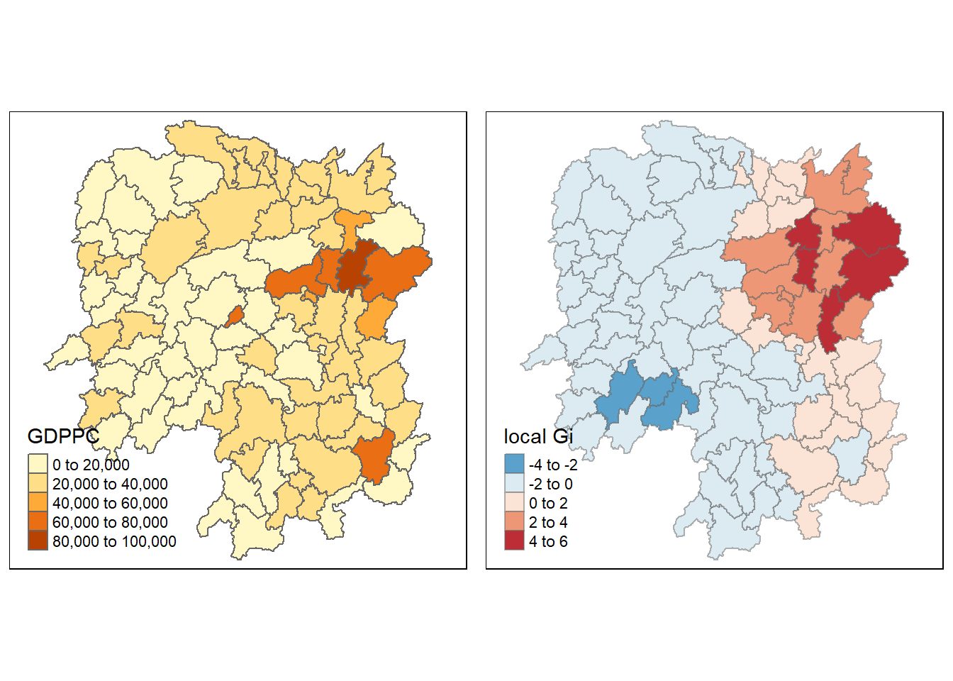
gdppc <- qtm(hunan, "GDPPC")

Gimap <-tm_shape(hunan.gi) +
  tm_fill(col = "gstat_fixed", 
          style = "pretty",
          palette="-RdBu",
          title = "local Gi") +
  tm_borders(alpha = 0.5)

tmap_arrange(gdppc, Gimap, asp=1, ncol=2)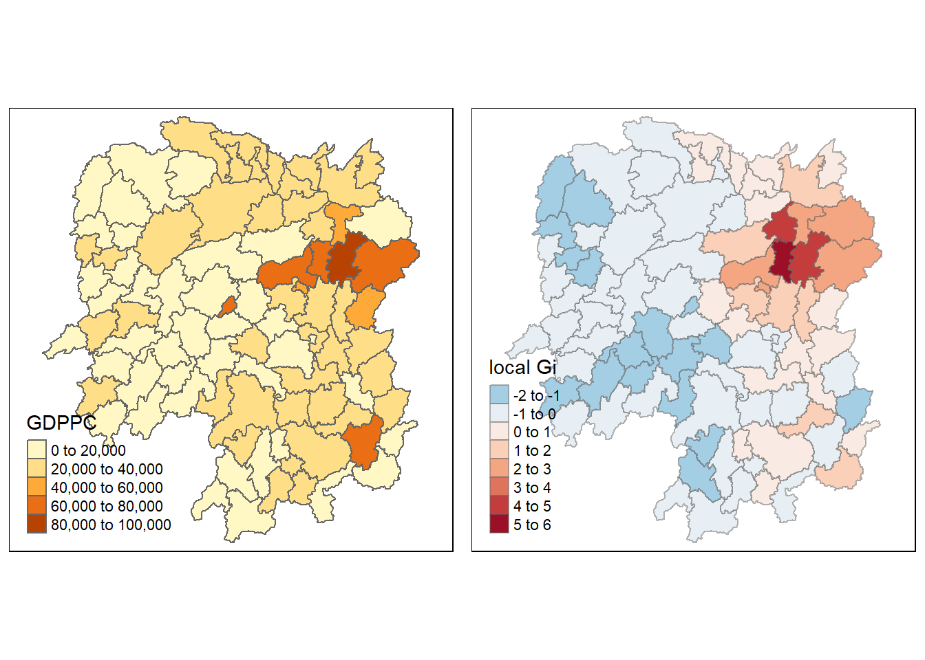

Gi statistics using adaptive distance

fips <- order(hunan$County)
gi.adaptive <- localG(hunan$GDPPC, knn_lw)
hunan.gi <- cbind(hunan, as.matrix(gi.adaptive)) %>%
  rename(gstat_adaptive = as.matrix.gi.adaptive.)

Mapping Gi values with adaptive distance weights

gdppc<- qtm(hunan, "GDPPC")

Gimap <- tm_shape(hunan.gi) + 
  tm_fill(col = "gstat_adaptive", 
          style = "pretty", 
          palette="-RdBu", 
          title = "local Gi") + 
  tm_borders(alpha = 0.5)

tmap_arrange(gdppc, 
             Gimap, 
             asp=1, 
             ncol=2)