Introduction
Housing is an essential component of household wealth worldwide. Buying a housing has always been a major investment for most people. The price of housing is affected by many factors. Some of them are global in nature such as the general economy of a country or inflation rate. Others can be more specific to the properties themselves. These factors can be further divided to structural and locational factors. Structural factors are variables related to the property themselves such as the size, fitting, and tenure of the property. Locational factors are variables related to the neighbourhood of the properties such as proximity to childcare centre, public transport service and shopping centre.
Conventional, housing resale prices predictive models were built by using Ordinary Least Square (OLS) Geographical Weighted Models were introduced for calibrating predictive model for housing resale prices.
We are now going to predict HDB resale prices at the sub-market level (i.e. HDB 5-room) The predictive models are built using by using conventional OLS method and GWR method, and we will also be comparing the performance of the conventional OLS method versus the geographical weighted methods.
Installing packages
:: p_load (olsrr, corrplot, ggpubr, sf, spdep, GWmodel, tmap, tidyverse, gtsummary, tidymodels, SpatialML, devtools, rsample, jsonlite, units, matrixStats, ranger, Metrics)
package 'tidymodels' successfully unpacked and MD5 sums checked
The downloaded binary packages are in
C:\Users\howxi\AppData\Local\Temp\RtmpMvPbeM\downloaded_packages
Importing data
Consisting of the structural factors:
HDB resale data (aspatial) - obtained from here
<- read_csv ("data/resale/resale-flat-prices-based-on-registration-date-from-jan-2017-onwards.csv" )
Locational factors: Master Plan Singapore 2019 (geospatial) - Provided by Prof Kam
= st_read (dsn = "data/mpsz" , layer = "MPSZ-2019" )
Reading layer `MPSZ-2019' from data source
`C:\xinyeehow\IS415-GAA\Take-Home_Ex\Take-Home_Ex03\data\mpsz'
using driver `ESRI Shapefile'
Simple feature collection with 332 features and 6 fields
Geometry type: MULTIPOLYGON
Dimension: XY
Bounding box: xmin: 103.6057 ymin: 1.158699 xmax: 104.0885 ymax: 1.470775
Geodetic CRS: WGS 84
<- mpsz %>% st_transform (crs = 3414 )
MRT Stations (geospatial) - obtained from here
= st_read (dsn = "data/TrainStation" , layer = "RapidTransitSystemStation" )
Reading layer `RapidTransitSystemStation' from data source
`C:\xinyeehow\IS415-GAA\Take-Home_Ex\Take-Home_Ex03\data\TrainStation'
using driver `ESRI Shapefile'
Simple feature collection with 220 features and 4 fields
Geometry type: POLYGON
Dimension: XY
Bounding box: xmin: 6068.209 ymin: 27478.44 xmax: 45377.5 ymax: 47913.58
Projected CRS: SVY21
<- mrt %>% st_transform (crs = 3414 )
<- mrt %>% st_cast ("MULTIPOLYGON" ) %>% st_make_valid ()
Bus stops (geospatial) - obtained from here
= st_read (dsn = "data/BusStop" , layer = "BusStop" )
Reading layer `BusStop' from data source
`C:\xinyeehow\IS415-GAA\Take-Home_Ex\Take-Home_Ex03\data\BusStop'
using driver `ESRI Shapefile'
Simple feature collection with 5159 features and 3 fields
Geometry type: POINT
Dimension: XY
Bounding box: xmin: 3970.122 ymin: 26482.1 xmax: 48284.56 ymax: 52983.82
Projected CRS: SVY21
<- busstop %>% st_transform (crs = 3414 )
Eldercare (geospatial) - obtained from here
= st_read (dsn = "data/eldercare" , layer = "ELDERCARE" )
Reading layer `ELDERCARE' from data source
`C:\xinyeehow\IS415-GAA\Take-Home_Ex\Take-Home_Ex03\data\eldercare'
using driver `ESRI Shapefile'
Simple feature collection with 133 features and 18 fields
Geometry type: POINT
Dimension: XY
Bounding box: xmin: 14481.92 ymin: 28218.43 xmax: 41665.14 ymax: 46804.9
Projected CRS: SVY21
<- eldercare %>% st_transform (crs = 3414 )
Childcare (geospatial) - obtained from here
= st_read (dsn = "data/childcare" , layer = "ChildcareServices" )
Reading layer `ChildcareServices' from data source
`C:\xinyeehow\IS415-GAA\Take-Home_Ex\Take-Home_Ex03\data\childcare'
using driver `ESRI Shapefile'
Simple feature collection with 1545 features and 2 fields
Geometry type: POINT
Dimension: XYZ
Bounding box: xmin: 11203.01 ymin: 25667.6 xmax: 45404.24 ymax: 49300.88
z_range: zmin: 0 zmax: 0
Projected CRS: SVY21 / Singapore TM
<- childcare %>% st_transform (crs = 3414 )
Primary schools - obtained from here , geocoded into shape file
<- st_read (dsn = "data/Education" , layer = "education" )
Reading layer `education' from data source
`C:\xinyeehow\IS415-GAA\Take-Home_Ex\Take-Home_Ex03\data\Education'
using driver `ESRI Shapefile'
Simple feature collection with 342 features and 15 fields
Geometry type: POINT
Dimension: XY
Bounding box: xmin: 103.7736 ymin: 1.276406 xmax: 103.8823 ymax: 1.427265
Geodetic CRS: WGS 84
Selecting primary schools only
<- subset (schools, mainlevel_ == "PRIMARY" | mainlevel_ == "MIXED LEVELS" )
Transforming into sf object
<- st_as_sf (schools, coords = c ("Longitude" , "Latitude" ), crs= 4326 ) %>% st_transform (crs = 3414 )
Good primary schools - obtained list of top 10 primary schools with the factors’ weightage included as well
<- read_csv ("data/Education/Good Schools.csv" )
Merging location information with school directory
<- left_join (good_schools, schools, by = c ("School" = "school_nam" ))
Transforming into sf object
<- st_as_sf (good_schools, coords = c ("Longitude" , "Latitude" ), crs= 4326 ) %>% st_transform (crs = 3414 )
Foodcourts/hawkers, Parks, Malls, and Supermarkets data obtained and extracted from here
= st_read (dsn = "data/singapore" , layer = "Singapore_POIS" )
Reading layer `Singapore_POIS' from data source
`C:\xinyeehow\IS415-GAA\Take-Home_Ex\Take-Home_Ex03\data\singapore'
using driver `ESRI Shapefile'
Simple feature collection with 18687 features and 4 fields
Geometry type: POINT
Dimension: XY
Bounding box: xmin: 3699.08 ymin: 22453.07 xmax: 52883.86 ymax: 50153.8
Projected CRS: SVY21 / Singapore TM
<- singapore %>% st_transform (crs = 3414 )
Subsetting foodcourts and hawkers
<- subset (singapore, fclass == "food_court" )
Parks
<- subset (singapore, fclass == "park" )
Shopping malls
<- subset (singapore, fclass == "mall" )
Supermarkets
<- subset (singapore, fclass == "supermarket" )
Central Business District - Setting the CBD to be at Downtown Core for this analysis’ purpose
<- 1.287953 <- 103.851784 <- data.frame (lat, lng) %>% st_as_sf (coords = c ("lng" , "lat" ), crs= 4326 ) %>% st_transform (crs= 3414 )
Filtering and cleaning data
Resale Flats (looking at 5 rooms between 1st January 2021 to 31st December 2022, since it’s more ideal for families)
<- resale %>% filter (flat_type == "5 ROOM" ) %>% filter (month >= "2021-01" & month <= "2022-12" )
Now, we need to retrieve postal codes using OneMap API in order to get the longitude and latitude values
Transforming ST. to SAINT to match OneMap’s API
$ street_name <- gsub ("ST \\ ." , "SAINT" , resale$ street_name)
Replacing NA values with 0
$ remaining_lease[is.na (resale$ remaining_lease)] <- 0
Setting up OneMap’s API
library (httr)<- function (block, streetname) {<- "https://developers.onemap.sg/commonapi/search" <- paste (block, streetname, sep = " " )<- list ("searchVal" = address, "returnGeom" = "Y" ,"getAddrDetails" = "N" ,"pageNum" = "1" )<- GET (base_url, query = query)<- content (res, as= "text" )<- fromJSON (restext) %>% %>% select (results.LATITUDE, results.LONGITUDE)return (output)
Geocoding latitude and longitude values
$ LATITUDE <- 0 $ LONGITUDE <- 0 for (i in 1 : nrow (resale)){<- geocode (resale[i, 4 ], resale[i, 5 ])$ LATITUDE[i] <- temp_output$ results.LATITUDE$ LONGITUDE[i] <- temp_output$ results.LONGITUDEwrite.csv (resale, "data/resale/resale.csv" )
Bringing in previously ran outputs
<- read_csv ("data/resale/resale.csv" )
Transforming remaining lease column into numeric values
<- str_split (resale$ remaining_lease, " " )for (i in 1 : length (str_list)) {if (length (unlist (str_list[i])) > 2 ) {<- as.numeric (unlist (str_list[i])[1 ])<- as.numeric (unlist (str_list[i])[3 ])$ remaining_lease[i] <- year + round (month/ 12 , 2 )else {<- as.numeric (unlist (str_list[i])[1 ])$ remaining_lease[i] <- year
Transforming into sf object and into desired projection
<- st_as_sf (resale, coords = c ("LONGITUDE" , "LATITUDE" ), crs= 4326 ) %>% st_transform (crs = 3414 )
Proximity Distance Calculation
<- function (df1, df2, varname) {<- st_distance (df1, df2) %>% drop_units ()<- rowMins (dist_matrix)return (df1)
<- proximity (resale_sf, cbd_sf, "PROX_CBD" ) %>% proximity (., childcare, "PROX_CHILDCARE" ) %>% proximity (., eldercare, "PROX_ELDERCARE" ) %>% proximity (., foodcourts, "PROX_FOODCOURT" ) %>% proximity (., mrt, "PROX_MRT" ) %>% proximity (., busstop, "PROX_BUSSTOP" ) %>% proximity (., parks, "PROX_PARK" ) %>% proximity (., good_schools_sf, "PROX_TOPPRISCH" ) %>% proximity (., malls, "PROX_MALL" ) %>% proximity (., supermarkets, "PROX_SPRMKT" ) %>% proximity (., schools_sf, "PROX_PRISCH" )
Facility count within radius
<- function (df1, df2, varname, radius) {<- st_distance (df1, df2) %>% drop_units () %>% as.data.frame ()<- rowSums (dist_matrix <= radius)return (df1)
<- num_radius (resale_sf, childcare, "NUM_CHILDCARE" , 350 ) %>% num_radius (., busstop, "NUM_BUSSTOP" , 350 ) %>% num_radius (., schools_sf, "NUM_PRISCH" , 1000 )
Saving dataset
<- resale_sf %>% mutate () %>% rename ("AREA_SQM" = "floor_area_sqm" , "LEASE_YRS" = "remaining_lease" , "PRICE" = "resale_price" ) %>% relocate (` PRICE ` )
st_write (resale_sf, "data/resale/resale_final.shp" )
Exploratory Data Analysis (EDA)
Bringing in saved layer
= st_read (dsn = "data/resale" , layer = "resale_final" )
Reading layer `resale_final' from data source
`C:\xinyeehow\IS415-GAA\Take-Home_Ex\Take-Home_Ex03\data\resale'
using driver `ESRI Shapefile'
Simple feature collection with 14519 features and 26 fields
Geometry type: POINT
Dimension: XY
Bounding box: xmin: 6958.193 ymin: 28157.26 xmax: 42645.18 ymax: 48741.06
Projected CRS: SVY21 / Singapore TM
Converting LEASE info into numeric format from string format
$ LEASE_Y <- as.numeric (resale_sf$ LEASE_Y)
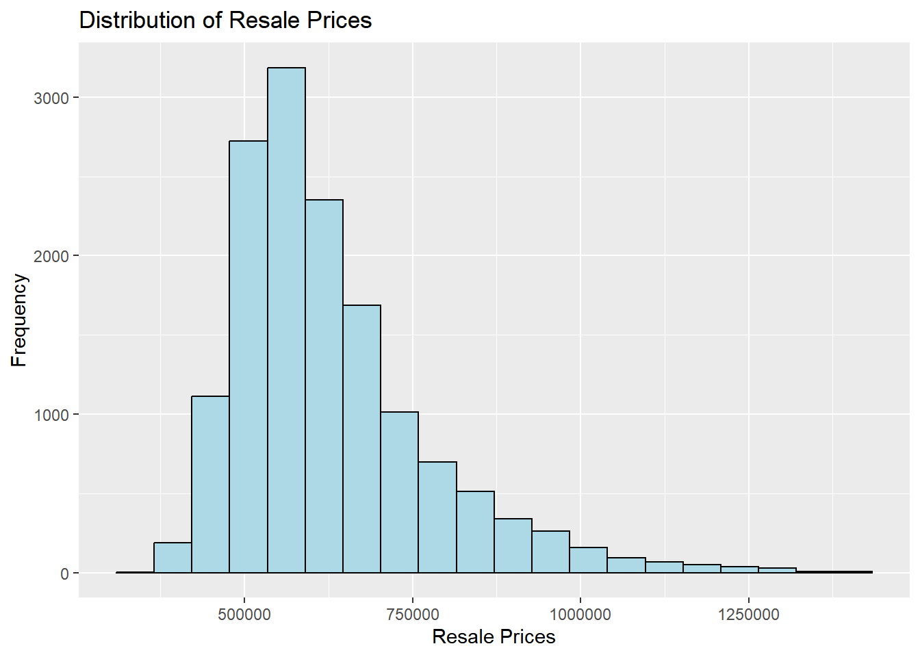
Distribution of selling prices of 5-room flats
ggplot (data= resale_sf, aes (x= ` PRICE ` )) + geom_histogram (bins= 20 , color= "black" , fill= "light blue" ) + labs (title = "Distribution of Resale Prices" ,x = "Resale Prices" ,y = 'Frequency' )
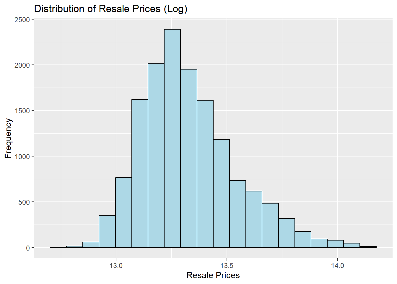
We see that the distribution is right-skewed. We will now use log-transformation to normalise the skewness
<- resale_sf %>% mutate (` LOG_PRICE ` = log (PRICE))ggplot (data = resale_sf, aes (x= ` LOG_PRICE ` )) + geom_histogram (bins= 20 , color= "black" , fill= "light blue" ) + labs (title = "Distribution of Resale Prices (Log)" ,x = "Resale Prices" ,y = 'Frequency' )
We can still see that the distribution is right skewed. That could mean that there are a lot of outliers with much higher transaction prices.
Min. 1st Qu. Median Mean 3rd Qu. Max.
350000 528000 595000 627297 690000 1418000
Our conclusion is confirmed by the statistics above.
Plotting the locations of the transactions
tmap_mode ("view" )tmap_options (check.and.fix = TRUE )tm_shape (resale_sf) + tm_dots (col = "PRICE" ,alpha = 0.6 ,style= "quantile" ) + # sets minimum zoom level to 11, sets maximum zoom level to 14 tm_view (set.zoom.limits = c (11 ,14 ))
From the plot above, we can conclude that the areas in the south and central of Singapore tend to have higher resale transactions for 5-room flats.
Linear regression
Simple linear regression model with price as our dependent variable and area_sqm as our independent variable
<- lm (formula= PRICE ~ AREA_SQ, data = resale_sf)
Call:
lm(formula = PRICE ~ AREA_SQ, data = resale_sf)
Residuals:
Min 1Q Median 3Q Max
-277295 -99351 -32417 62672 790677
Coefficients:
Estimate Std. Error t value Pr(>|t|)
(Intercept) 6.266e+05 1.953e+04 32.092 <2e-16 ***
AREA_SQ 5.565e+00 1.660e+02 0.034 0.973
---
Signif. codes: 0 '***' 0.001 '**' 0.01 '*' 0.05 '.' 0.1 ' ' 1
Residual standard error: 146100 on 14517 degrees of freedom
Multiple R-squared: 7.741e-08, Adjusted R-squared: -6.881e-05
F-statistic: 0.001124 on 1 and 14517 DF, p-value: 0.9733
R-squared value obtained is less than 0.001, which means the model is not useful in predicting the price of 5-room models.
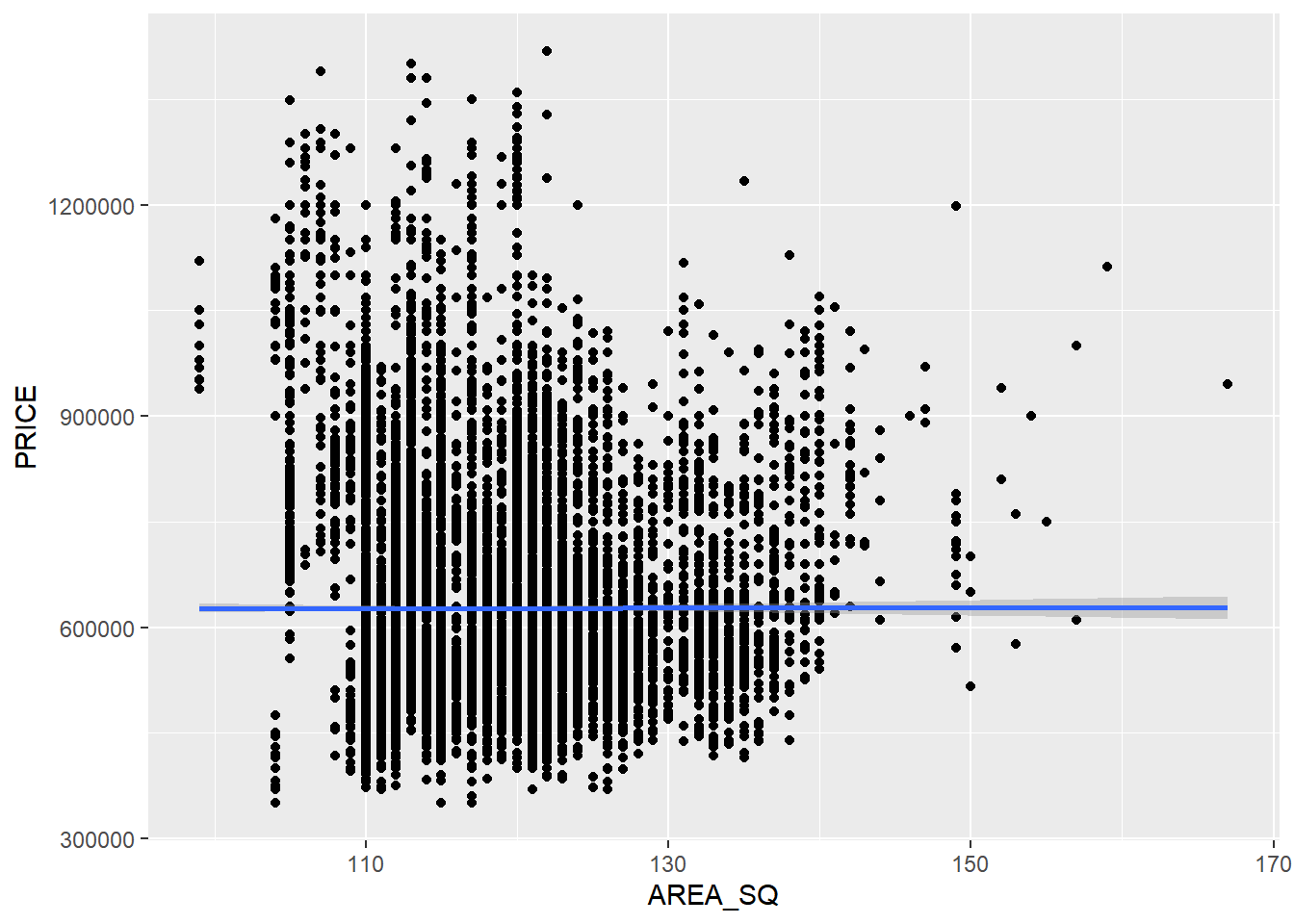
Best fit line graph
ggplot (data= resale_sf, aes (x= ` AREA_SQ ` , y= ` PRICE ` )) + geom_point () + geom_smooth (method = lm)
Values are too varied, not reliable!
Now let’s build a multiple regression model
Multiple regression model
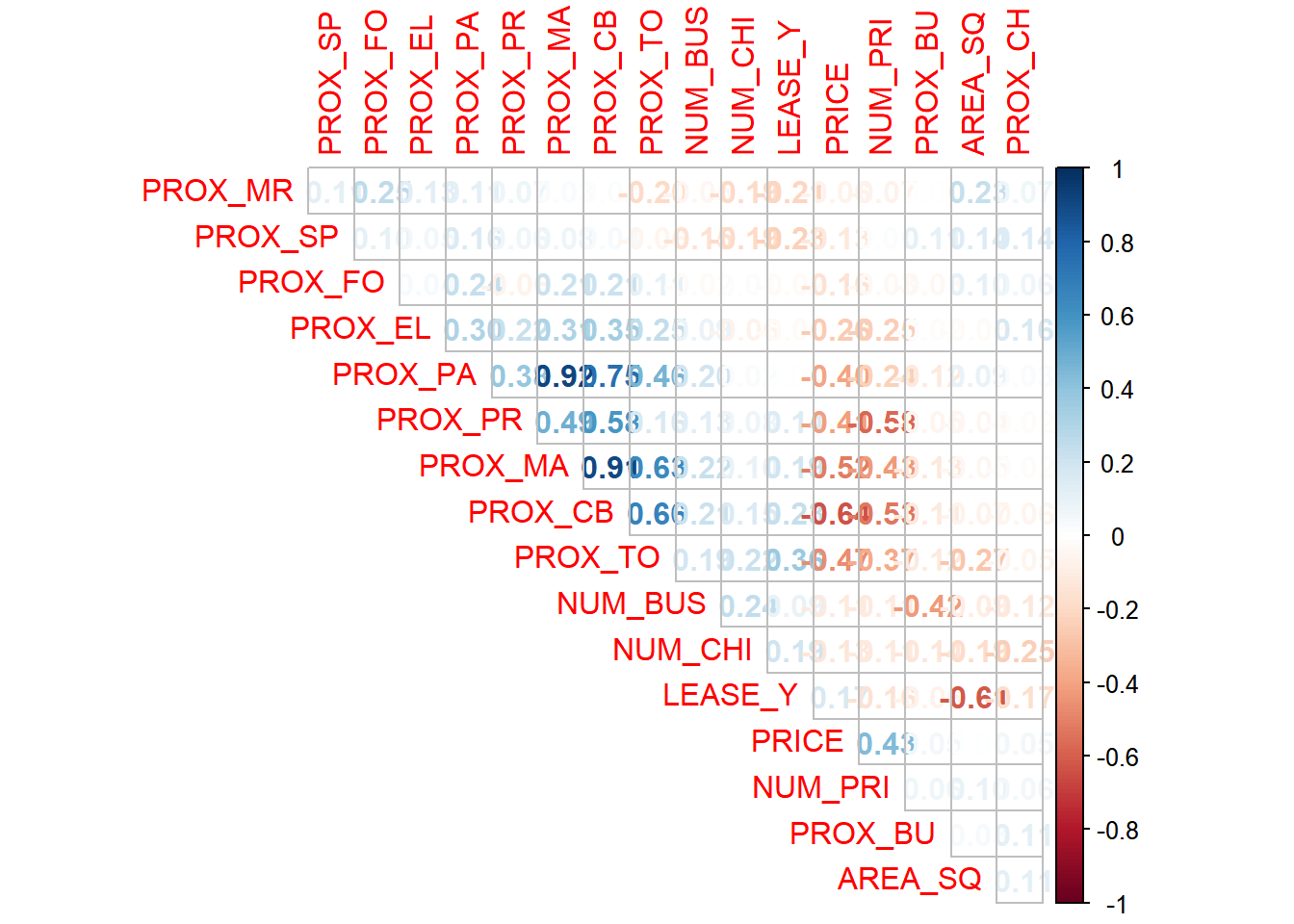
Plotting correlation plot to determine multicollinearity
<- resale_sf %>% st_drop_geometry () %>% :: select (c (1 ,9 ,12 : 26 ))
corrplot (cor (resale_nogeom_sf), diag = FALSE , order = "AOE" ,t1.pos = "td" ,t1.cex = 0.5 ,method = "number" ,type = "upper" )
High correlation between malls and CBD, so let’s proceed to drop them
<- c ("PROX_MA" )<- resale_sf[ , ! (names (resale_sf) %in% drops)]
<- c ("PROX_CB" )<- resale_sf[ , ! (names (resale_sf) %in% drops)]
Splitting test and train data
Setting train data to be 6 months from March 2022 to September 2022 to reduce computational time, test data to be from October to December 2022
<- resale_sf %>% filter (month >= "2022-03" & month <= "2022-09" )
<- resale_sf %>% filter (month >= "2022-10" & month <= "2022-12" )
write_rds (train_data, "data/model/train_data.rds" )write_rds (test_data, "data/model/test_data.rds" )
Retrieving stored data
<- read_rds ("data/model/train_data.rds" )<- read_rds ("data/model/test_data.rds" )
Non-spatial multiple regression model
<- lm (formula = PRICE ~ AREA_SQ + LEASE_Y + stry_rn + + PROX_EL + PROX_FO + PROX_MR + + PROX_PA + PROX_TO + PROX_SP + + NUM_PRI + NUM_CHI + NUM_BUS, data = train_data)summary (resale_mlr)
Call:
lm(formula = PRICE ~ AREA_SQ + LEASE_Y + stry_rn + PROX_CH +
PROX_EL + PROX_FO + PROX_MR + PROX_BU + PROX_PA + PROX_TO +
PROX_SP + PROX_PR + NUM_PRI + NUM_CHI + NUM_BUS, data = train_data)
Residuals:
Min 1Q Median 3Q Max
-278723 -51153 -9787 41165 491620
Coefficients:
Estimate Std. Error t value Pr(>|t|)
(Intercept) -1.984e+05 3.506e+04 -5.660 1.62e-08 ***
AREA_SQ 5.105e+03 2.264e+02 22.543 < 2e-16 ***
LEASE_Y 5.976e+03 1.411e+02 42.357 < 2e-16 ***
stry_rn04 TO 06 2.416e+04 4.157e+03 5.811 6.69e-09 ***
stry_rn07 TO 09 4.215e+04 4.149e+03 10.161 < 2e-16 ***
stry_rn10 TO 12 5.129e+04 4.356e+03 11.776 < 2e-16 ***
stry_rn13 TO 15 6.467e+04 4.806e+03 13.456 < 2e-16 ***
stry_rn16 TO 18 9.350e+04 5.987e+03 15.616 < 2e-16 ***
stry_rn19 TO 21 1.265e+05 7.922e+03 15.968 < 2e-16 ***
stry_rn22 TO 24 1.443e+05 9.338e+03 15.451 < 2e-16 ***
stry_rn25 TO 27 1.810e+05 1.184e+04 15.290 < 2e-16 ***
stry_rn28 TO 30 2.111e+05 1.650e+04 12.798 < 2e-16 ***
stry_rn31 TO 33 2.926e+05 2.335e+04 12.530 < 2e-16 ***
stry_rn34 TO 36 2.701e+05 2.343e+04 11.527 < 2e-16 ***
stry_rn37 TO 39 3.127e+05 3.036e+04 10.299 < 2e-16 ***
stry_rn40 TO 42 5.116e+05 5.635e+04 9.079 < 2e-16 ***
stry_rn46 TO 48 6.390e+05 4.602e+04 13.885 < 2e-16 ***
PROX_CH 6.399e+01 1.222e+01 5.238 1.71e-07 ***
PROX_EL -2.445e+00 2.089e+00 -1.170 0.2419
PROX_FO -5.444e+01 4.631e+00 -11.757 < 2e-16 ***
PROX_MR -1.671e+01 3.711e+00 -4.504 6.84e-06 ***
PROX_BU -2.280e+01 2.354e+01 -0.968 0.3330
PROX_PA -1.962e+00 4.733e-01 -4.146 3.46e-05 ***
PROX_TO -2.680e+01 7.754e-01 -34.561 < 2e-16 ***
PROX_SP -4.254e+01 8.434e+00 -5.044 4.76e-07 ***
PROX_PR -1.421e+01 6.183e-01 -22.983 < 2e-16 ***
NUM_PRI 1.477e+04 2.016e+03 7.326 2.84e-13 ***
NUM_CHI -3.171e+03 6.588e+02 -4.813 1.54e-06 ***
NUM_BUS 1.112e+03 4.683e+02 2.374 0.0176 *
---
Signif. codes: 0 '***' 0.001 '**' 0.01 '*' 0.05 '.' 0.1 ' ' 1
Residual standard error: 79270 on 4084 degrees of freedom
Multiple R-squared: 0.6994, Adjusted R-squared: 0.6974
F-statistic: 339.4 on 28 and 4084 DF, p-value: < 2.2e-16
write_rds (resale_mlr, "data/model/resale_mlr.rds" )
Prediction using OLS method
<- lm (formula = PRICE ~ AREA_SQ + LEASE_Y + + PROX_EL + PROX_FO + PROX_MR + + PROX_PA + PROX_TO + PROX_SP + + NUM_PRI + NUM_CHI + NUM_BUS,data = resale_nogeom_sf)ols_regress (resale_mlr)
Model Summary
----------------------------------------------------------------------
R 0.734 RMSE 99329.030
R-Squared 0.538 Coef. Var 15.834
Adj. R-Squared 0.538 MSE 9866256274.328
Pred R-Squared 0.536 MAE 74867.602
----------------------------------------------------------------------
RMSE: Root Mean Square Error
MSE: Mean Square Error
MAE: Mean Absolute Error
ANOVA
--------------------------------------------------------------------------------
Sum of
Squares DF Mean Square F Sig.
--------------------------------------------------------------------------------
Regression 1.667916e+14 14 1.191368e+13 1207.518 0.0000
Residual 1.431002e+14 14504 9866256274.328
Total 3.098918e+14 14518
--------------------------------------------------------------------------------
Parameter Estimates
---------------------------------------------------------------------------------------------------
model Beta Std. Error Std. Beta t Sig lower upper
---------------------------------------------------------------------------------------------------
(Intercept) 59297.199 22875.201 2.592 0.010 14458.887 104135.512
AREA_SQ 3188.567 147.439 0.159 21.626 0.000 2899.568 3477.566
LEASE_Y 6172.896 93.995 0.507 65.672 0.000 5988.654 6357.139
PROX_CH 116.081 7.232 0.096 16.051 0.000 101.905 130.257
PROX_EL -5.466 1.406 -0.024 -3.888 0.000 -8.221 -2.711
PROX_FO -62.421 3.168 -0.122 -19.704 0.000 -68.631 -56.211
PROX_MR -14.833 2.468 -0.038 -6.009 0.000 -19.671 -9.995
PROX_BU -41.891 15.841 -0.017 -2.644 0.008 -72.942 -10.840
PROX_PA 0.273 0.312 0.007 0.876 0.381 -0.338 0.884
PROX_TO -31.073 0.496 -0.499 -62.695 0.000 -32.044 -30.101
PROX_SP -40.147 5.615 -0.043 -7.150 0.000 -51.152 -29.141
PROX_PR -17.507 0.404 -0.337 -43.285 0.000 -18.300 -16.714
NUM_PRI 16970.092 1359.735 0.095 12.480 0.000 14304.838 19635.346
NUM_CHI -3493.926 444.310 -0.049 -7.864 0.000 -4364.830 -2623.023
NUM_BUS 413.029 312.420 0.009 1.322 0.186 -199.353 1025.412
---------------------------------------------------------------------------------------------------
<- predict (resale_mlr, data = train_data)summary (resale_mlr_pred)
Min. 1st Qu. Median Mean 3rd Qu. Max.
319799 558783 615654 627297 681438 1034589
tbl_regression (resale_mlr, intercept = TRUE )
Characteristic Beta 95% CI p-value
(Intercept)
59,297
14,459, 104,136
0.010 AREA_SQ
3,189
2,900, 3,478
<0.001 LEASE_Y
6,173
5,989, 6,357
<0.001 PROX_CH
116
102, 130
<0.001 PROX_EL
-5.5
-8.2, -2.7
<0.001 PROX_FO
-62
-69, -56
<0.001 PROX_MR
-15
-20, -10
<0.001 PROX_BU
-42
-73, -11
0.008 PROX_PA
0.27
-0.34, 0.88
0.4 PROX_TO
-31
-32, -30
<0.001 PROX_SP
-40
-51, -29
<0.001 PROX_PR
-18
-18, -17
<0.001 NUM_PRI
16,970
14,305, 19,635
<0.001 NUM_CHI
-3,494
-4,365, -2,623
<0.001 NUM_BUS
413
-199, 1,025
0.2
Checking for multicollinearity
Variables Tolerance VIF
1 AREA_SQ 0.5859146 1.706733
2 LEASE_Y 0.5332502 1.875292
3 PROX_CH 0.8832071 1.132237
4 PROX_EL 0.8088947 1.236255
5 PROX_FO 0.8316944 1.202365
6 PROX_MR 0.7888073 1.267737
7 PROX_BU 0.8100352 1.234514
8 PROX_PA 0.5376632 1.859900
9 PROX_TO 0.5026562 1.989431
10 PROX_SP 0.8626090 1.159274
11 PROX_PR 0.5257821 1.901928
12 NUM_PRI 0.5466689 1.829261
13 NUM_CHI 0.8099186 1.234692
14 NUM_BUS 0.7442748 1.343590
Since none of the variables have a VIF value more than 10, we can conclude that there are no signs of multicollinearities among the variables.
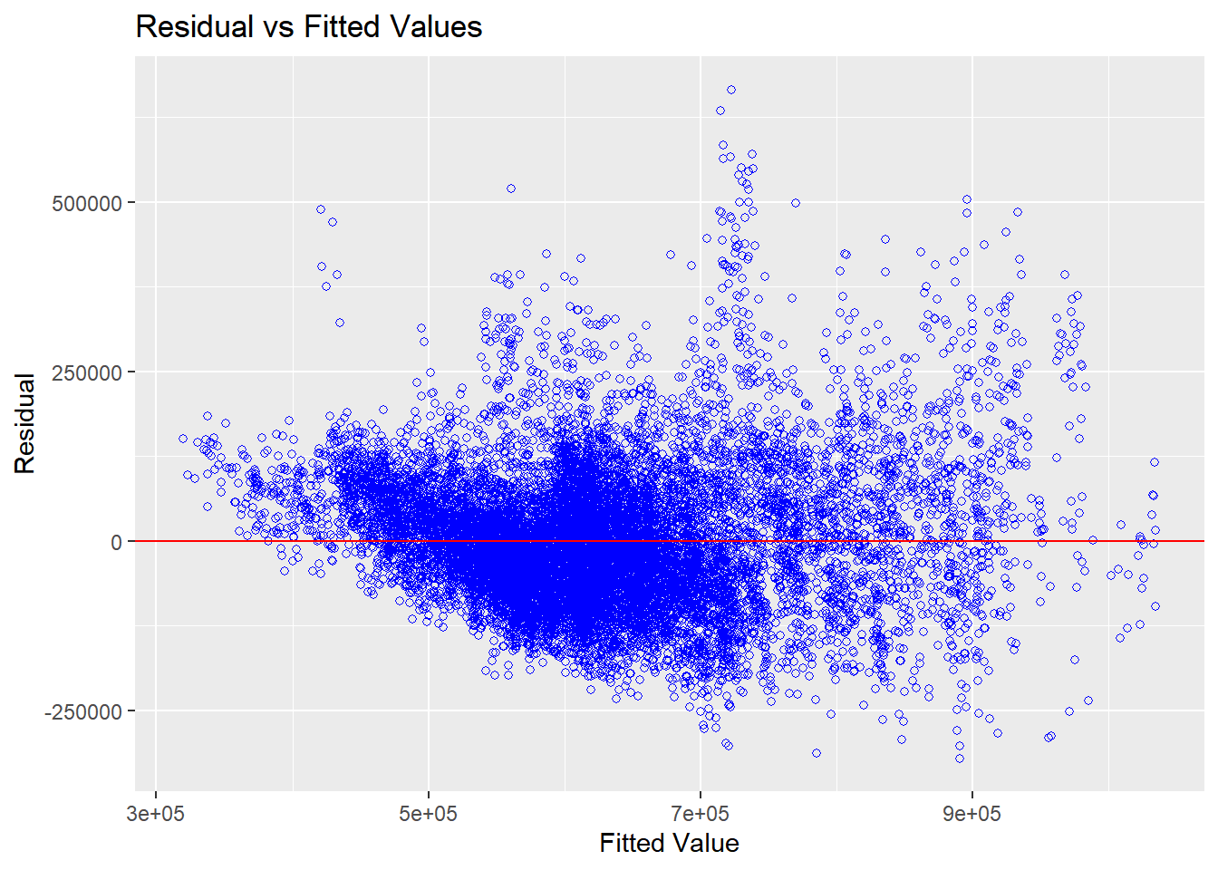
Test for non-linearity
ols_plot_resid_fit (resale_mlr)
We can observe that most of the points lies near the 0 line from the plot above, and we can conclude that the relationship between the independent and dependent variables are linear.
GRW Predictive method
Converting train data into spatial data
<- as_Spatial (train_data)
class : SpatialPointsDataFrame
features : 4113
extent : 6958.193, 42645.18, 28299.14, 48741.06 (xmin, xmax, ymin, ymax)
crs : +proj=tmerc +lat_0=1.36666666666667 +lon_0=103.833333333333 +k=1 +x_0=28001.642 +y_0=38744.572 +ellps=WGS84 +towgs84=0,0,0,0,0,0,0 +units=m +no_defs
variables : 25
names : PRICE, X___1, month, town, flt_typ, block, strt_nm, stry_rn, AREA_SQ, flt_mdl, ls_cmm_, LEASE_Y, PROX_CH, PROX_EL, PROX_FO, ...
min values : 4e+05, 7805, 2022-03, ANG MO KIO, 5 ROOM, 1, ADMIRALTY DR, 01 TO 03, 99, 3Gen, 1972, 49.25, 0.000104604717071, 0.001038255324477, 8.054189158654, ...
max values : 1418000, 14514, 2022-09, YISHUN, 5 ROOM, 9B, ZION RD, 46 TO 48, 159, Type S2, 2019, 96.08, 4567.62297455935, 8265.97091415839, 1904.41400290072, ...
<- train_data_sp %>% st_drop_geometry ()
Computing adaptive bandwidth
<- bw.gwr (PRICE ~ AREA_SQ + LEASE_Y + stry_rn + + PROX_EL + PROX_FO + PROX_MR + + PROX_PA + PROX_TO + PROX_SP + + NUM_PRI + NUM_CHI + NUM_BUS,data= train_data_sp,approach= "CV" ,kernel= "gaussian" ,adaptive= TRUE ,longlat= FALSE )
Saving bw_adaptive output
write_rds (bw_adaptive, file = "data/model/bw_adaptive.rds" )
Bringing in previously ran data
<- read_rds ("data/model/bw_adaptive.rds" )
Calculating GWR adaptive
<- gwr.basic (formula = PRICE ~ AREA_SQ + LEASE_Y + stry_rn + + PROX_EL + PROX_FO + PROX_MR + + PROX_PA + PROX_TO + PROX_SP + + NUM_PRI + NUM_CHI + NUM_BUS,data = train_data_sp,bw= bw_adaptive, kernel = 'gaussian' , adaptive= TRUE ,longlat = FALSE )write_rds (gwr_adaptive, "data/model/gwr_adaptive.rds" )
Bringing in previously ran outputs
<- read_rds ("data/model/gwr_adaptive.rds" )
***********************************************************************
* Package GWmodel *
***********************************************************************
Program starts at: 2023-03-19 22:36:43
Call:
gwr.basic(formula = PRICE ~ AREA_SQ + LEASE_Y + stry_rn + PROX_CH +
PROX_EL + PROX_FO + PROX_MR + PROX_BU + PROX_PA + PROX_TO +
PROX_SP + PROX_PR + NUM_PRI + NUM_CHI + NUM_BUS, data = train_data_sp,
bw = bw_adaptive, kernel = "gaussian", adaptive = TRUE, longlat = FALSE)
Dependent (y) variable: PRICE
Independent variables: AREA_SQ LEASE_Y stry_rn PROX_CH PROX_EL PROX_FO PROX_MR PROX_BU PROX_PA PROX_TO PROX_SP PROX_PR NUM_PRI NUM_CHI NUM_BUS
Number of data points: 9437
***********************************************************************
* Results of Global Regression *
***********************************************************************
Call:
lm(formula = formula, data = data)
Residuals:
Min 1Q Median 3Q Max
-313109 -59170 -5999 50243 570049
Coefficients:
Estimate Std. Error t value Pr(>|t|)
(Intercept) -9.914e+04 2.544e+04 -3.896 9.84e-05 ***
AREA_SQ 4.138e+03 1.635e+02 25.311 < 2e-16 ***
LEASE_Y 5.399e+03 1.044e+02 51.709 < 2e-16 ***
stry_rn04 TO 06 2.676e+04 3.013e+03 8.880 < 2e-16 ***
stry_rn07 TO 09 4.648e+04 3.036e+03 15.309 < 2e-16 ***
stry_rn10 TO 12 5.131e+04 3.111e+03 16.491 < 2e-16 ***
stry_rn13 TO 15 6.486e+04 3.493e+03 18.566 < 2e-16 ***
stry_rn16 TO 18 9.281e+04 4.355e+03 21.314 < 2e-16 ***
stry_rn19 TO 21 1.279e+05 5.930e+03 21.576 < 2e-16 ***
stry_rn22 TO 24 1.567e+05 6.739e+03 23.258 < 2e-16 ***
stry_rn25 TO 27 1.789e+05 8.933e+03 20.033 < 2e-16 ***
stry_rn28 TO 30 2.350e+05 1.276e+04 18.427 < 2e-16 ***
stry_rn31 TO 33 3.006e+05 1.629e+04 18.449 < 2e-16 ***
stry_rn34 TO 36 3.518e+05 1.750e+04 20.101 < 2e-16 ***
stry_rn37 TO 39 3.574e+05 1.821e+04 19.626 < 2e-16 ***
stry_rn40 TO 42 4.946e+05 2.448e+04 20.205 < 2e-16 ***
stry_rn43 TO 45 4.792e+05 5.060e+04 9.471 < 2e-16 ***
stry_rn46 TO 48 6.006e+05 3.925e+04 15.304 < 2e-16 ***
PROX_CH 1.050e+02 7.048e+00 14.895 < 2e-16 ***
PROX_EL -1.297e+00 1.530e+00 -0.847 0.3968
PROX_FO -4.704e+01 3.488e+00 -13.485 < 2e-16 ***
PROX_MR -1.652e+01 2.701e+00 -6.115 1.00e-09 ***
PROX_BU -2.470e+01 1.748e+01 -1.413 0.1578
PROX_PA -1.278e+00 3.434e-01 -3.721 0.0002 ***
PROX_TO -2.555e+01 5.552e-01 -46.015 < 2e-16 ***
PROX_SP -4.115e+01 6.150e+00 -6.691 2.34e-11 ***
PROX_PR -1.306e+01 4.506e-01 -28.988 < 2e-16 ***
NUM_PRI 1.682e+04 1.482e+03 11.351 < 2e-16 ***
NUM_CHI -2.497e+03 4.895e+02 -5.101 3.45e-07 ***
NUM_BUS 4.980e+02 3.415e+02 1.458 0.1448
---Significance stars
Signif. codes: 0 '***' 0.001 '**' 0.01 '*' 0.05 '.' 0.1 ' ' 1
Residual standard error: 87420 on 9407 degrees of freedom
Multiple R-squared: 0.6386
Adjusted R-squared: 0.6375
F-statistic: 573.2 on 29 and 9407 DF, p-value: < 2.2e-16
***Extra Diagnostic information
Residual sum of squares: 7.189156e+13
Sigma(hat): 87290.71
AIC: 241570.5
AICc: 241570.7
BIC: 232639
***********************************************************************
* Results of Geographically Weighted Regression *
***********************************************************************
*********************Model calibration information*********************
Kernel function: gaussian
Adaptive bandwidth: 235 (number of nearest neighbours)
Regression points: the same locations as observations are used.
Distance metric: Euclidean distance metric is used.
****************Summary of GWR coefficient estimates:******************
Min. 1st Qu. Median 3rd Qu. Max.
Intercept -3.0200e+06 -8.1228e+05 -2.9186e+05 3.5031e+03 3.6752e+06
AREA_SQ -4.4561e+03 2.6658e+03 4.0433e+03 5.7884e+03 1.5072e+04
LEASE_Y 2.0186e+02 4.9176e+03 6.1000e+03 7.2406e+03 1.0368e+04
stry_rn04.TO.06 1.0232e+04 1.8639e+04 2.3358e+04 2.8510e+04 4.4959e+04
stry_rn07.TO.09 2.5919e+04 3.6260e+04 4.2026e+04 5.1899e+04 9.0669e+04
stry_rn10.TO.12 2.8938e+04 4.3445e+04 4.9558e+04 6.2359e+04 9.5524e+04
stry_rn13.TO.15 3.7078e+04 5.1438e+04 6.0017e+04 7.6112e+04 1.3365e+05
stry_rn16.TO.18 -1.5579e+05 5.8940e+04 7.6080e+04 1.0657e+05 1.6322e+05
stry_rn19.TO.21 -2.9276e+05 7.3154e+04 9.1650e+04 1.2268e+05 3.6835e+05
stry_rn22.TO.24 -4.1194e+05 8.5428e+04 1.2067e+05 1.5303e+05 4.1617e+05
stry_rn25.TO.27 -6.4380e+05 7.7852e+04 1.2725e+05 1.6289e+05 7.1261e+05
stry_rn28.TO.30 -8.5810e+05 1.2028e+05 2.0355e+05 2.9042e+05 5.6957e+05
stry_rn31.TO.33 -9.1198e+05 1.2536e+05 2.1880e+05 3.1900e+05 1.2315e+06
stry_rn34.TO.36 -1.0388e+05 2.8378e+05 4.0355e+05 5.1603e+05 1.2906e+06
stry_rn37.TO.39 -1.3407e+05 2.4727e+05 3.3383e+05 4.8551e+05 1.2523e+06
stry_rn40.TO.42 -1.8271e+06 3.6314e+05 4.6673e+05 6.5058e+05 1.7713e+06
stry_rn43.TO.45 -3.3122e+06 3.6545e+05 5.4278e+05 7.0935e+05 3.0379e+06
stry_rn46.TO.48 -2.0366e+06 5.2511e+05 6.0480e+05 7.3673e+05 2.5576e+06
PROX_CH -2.4503e+02 -4.2375e+01 1.1423e+01 5.1692e+01 1.6033e+02
PROX_EL -6.8816e+01 -1.3846e+01 6.7214e+00 2.9319e+01 1.8220e+02
PROX_FO -1.3728e+02 -5.6427e+01 -3.5018e+01 -7.3794e+00 9.3581e+01
PROX_MR -1.8948e+02 -8.4182e+01 -5.0445e+01 -2.9165e+01 7.9122e+01
PROX_BU -3.8127e+02 -2.2305e+01 2.1902e+01 9.8272e+01 3.2268e+02
PROX_PA -2.9461e+02 -2.8777e+01 7.9209e+00 6.7292e+01 8.3100e+02
PROX_TO -9.1676e+02 -4.1495e+01 -3.7385e+00 5.3950e+01 9.0907e+02
PROX_SP -1.5798e+02 -4.9068e+01 -1.8385e+01 1.5569e+01 1.1211e+02
PROX_PR -6.3029e+02 -5.8135e+01 -4.9329e+00 2.0667e+01 2.5248e+02
NUM_PRI -1.5124e+06 -7.3391e+03 1.7045e+04 8.4198e+04 1.3702e+06
NUM_CHI -6.6886e+03 -1.0608e+03 8.3713e+02 2.6145e+03 1.7163e+04
NUM_BUS -6.8001e+03 -1.8350e+03 -2.9479e+02 1.3620e+03 5.9301e+03
************************Diagnostic information*************************
Number of data points: 9437
Effective number of parameters (2trace(S) - trace(S'S)): 583.0149
Effective degrees of freedom (n-2trace(S) + trace(S'S)): 8853.985
AICc (GWR book, Fotheringham, et al. 2002, p. 61, eq 2.33): 233134.1
AIC (GWR book, Fotheringham, et al. 2002,GWR p. 96, eq. 4.22): 232637.4
BIC (GWR book, Fotheringham, et al. 2002,GWR p. 61, eq. 2.34): 226864.4
Residual sum of squares: 2.677563e+13
R-square value: 0.865401
Adjusted R-square value: 0.856537
***********************************************************************
Program stops at: 2023-03-19 22:44:19
R square value is 0.8565, which means it can predict around 85% of the data. This is pretty high
Coordinates data
Preparing coordinates data
<- st_coordinates (train_data)<- st_coordinates (test_data)
Saving coordinates data
<- write_rds (coords_train, "data/model/coords_train.rds" )<- write_rds (coords_test, "data/model/coords_test.rds" )
Bringing in saved coordinates data
<- read_rds ("data/model/coords_train.rds" )<- read_rds ("data/model/coords_test.rds" )
Dropping geometric fields - to prep for random forest data
<- train_data %>% st_drop_geometry ()
Saving output
write_rds (train_data_nogeom, "data/model/train_data_nogeom.rds" )
Bringing in saved train data
<- read_rds ("data/model/train_data_nogeom.rds" )
Calibrating Random Forest Model
Using ranger package
set.seed (1234 )<- ranger (PRICE ~ AREA_SQ + LEASE_Y + stry_rn + + PROX_EL + PROX_FO + PROX_MR + + PROX_PA + PROX_TO + PROX_SP + + NUM_PRI + NUM_CHI + NUM_BUS,data= train_data_nogeom)
Ranger result
Call:
ranger(PRICE ~ AREA_SQ + LEASE_Y + stry_rn + PROX_CH + PROX_EL + PROX_FO + PROX_MR + PROX_BU + PROX_PA + PROX_TO + PROX_SP + PROX_PR + NUM_PRI + NUM_CHI + NUM_BUS, data = train_data_nogeom)
Type: Regression
Number of trees: 500
Sample size: 4113
Number of independent variables: 15
Mtry: 3
Target node size: 5
Variable importance mode: none
Splitrule: variance
OOB prediction error (MSE): 1912577810
R squared (OOB): 0.9078936
Calculating ranger bandwidth
<- grf.bw (formula = PRICE ~ AREA_SQ + LEASE_Y + stry_rn + + PROX_EL + PROX_FO + PROX_MR + + PROX_PA + PROX_TO + PROX_SP + + NUM_PRI + NUM_CHI + NUM_BUS,data = train_data_nogeom,kernel = "adaptive" ,trees = 30 ,coords = coords_trainwrite_rds (gwRF_bw, "data/model/gwRF_bw.rds" )
Bringing in previously saved outputs
<- read_rds ("data/model/gwRF_bw.rds" )
Calibrating Geographical Random Forest Model Using SpatialML package
set.seed (1234 )<- grf (formula = PRICE ~ AREA_SQ + LEASE_Y + stry_rn + + PROX_EL + PROX_FO + PROX_MR + + PROX_PA + PROX_TO + PROX_SP + + NUM_PRI + NUM_CHI + NUM_BUS,dframe= train_data_nogeom, bw= bw_adaptive,kernel= "adaptive" ,ntree = 30 ,coords= coords_train)write_rds (gwRF_adaptive, "data/model/gwRF_adaptive.rds" )
Bringing in previously ran outputs
<- read_rds ("data/model/gwRF_adaptive.rds" )
Predicting by using test data
Preparing test data (drop geometries first)
<- cbind (test_data, coords_test) %>% st_drop_geometry ()
Predicting with test data
<- predict.grf (gwRF_adaptive, x.var.name= "X" ,y.var.name= "Y" , local.w= 1 ,global.w= 0 )<- write_rds (gwRF_pred, "data/model/GRF_pred.rds" )
Converting predicted output into a dataframe
<- read_rds ("data/model/GRF_pred.rds" )<- as.data.frame (GRF_pred)
Appending predicted values into test data
<- cbind (test_data, GRF_pred_df)
Saving values
write_rds (test_data_p, "data/model/test_data_p.rds" )
Bringing in previously ran results
<- read_rds ("data/model/test_data_p.rds" )
Calculating Root Mean Square Error
$ GRF_pred <- as.numeric (test_data_p$ GRF_pred)
rmse (test_data_p$ PRICE, $ GRF_pred)
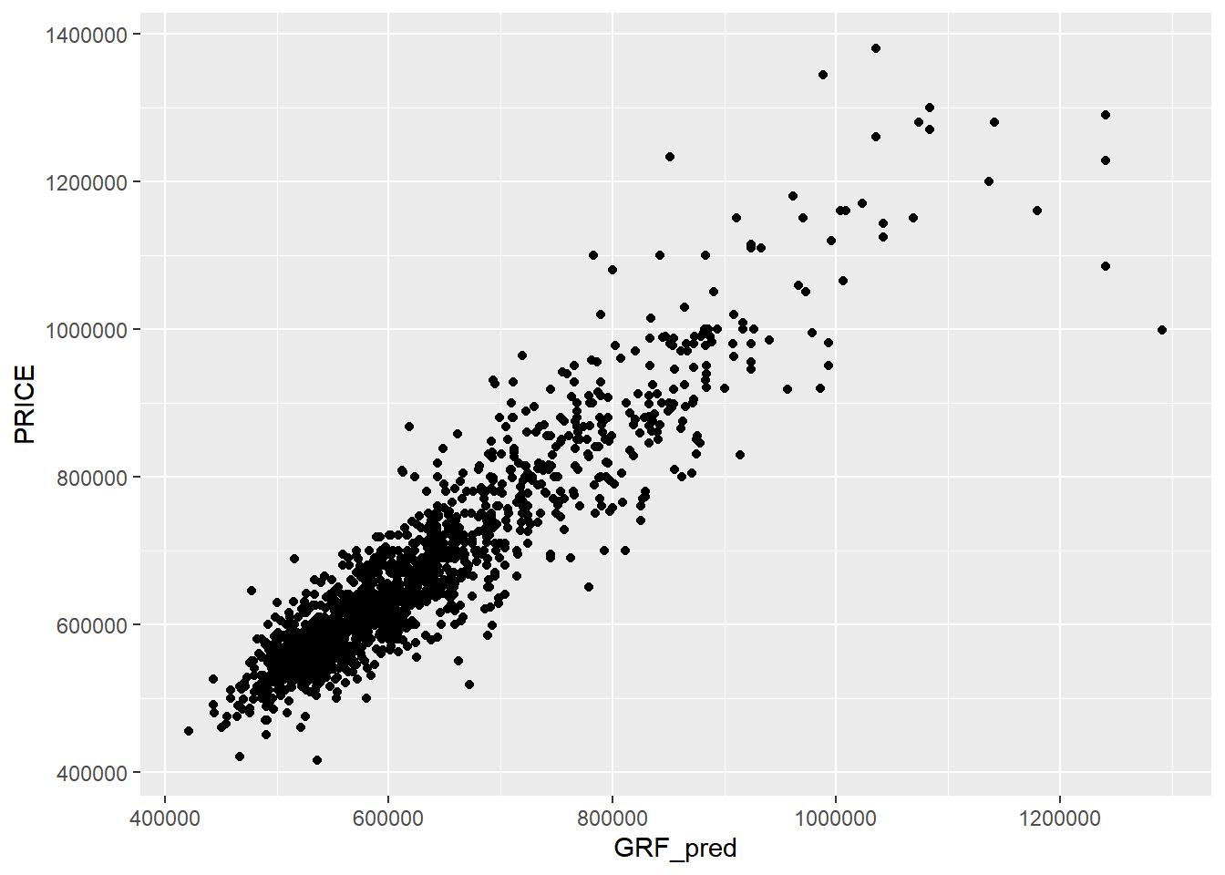
Visualising predicted values
ggplot (data = test_data_p,aes (x = GRF_pred,y = PRICE)) + geom_point ()
A better predictive model should have the scatter point close to the diagonal line. In this case, the predictive model seems to be working very well until the $900,000 mark. The scatter plot also highlighted the presence of outliers in the model, for the points above the $900,001 mark. This shows that majority of the 5-room HDB units in Singapore are priced below $900,000 and those looking to purchase 5-room units above $900,000 should proceed with caution as the price will be above valuation.
References
With guidance from Prof Kam Tin Seong and senior Megan Sim